MSA
The MSA module of MIToS has utilities for working with Multiple Sequence Alignments of protein Sequences (MSA).
using MIToS.MSA # to load the MSA moduleFeatures
- Read and write MSAs in
Stockholm,FASTA,A3M,A2M,PIR,ClustalorRawformat. - Handle MSA annotations.
- Edit the MSA, e.g. delete columns or sequences, change sequence order, shuffling...
- Keep track of positions and annotations after modifications on the MSA.
- Describe an MSA, e.g. mean percent identity, sequence coverage, gap percentage...
- Sequence clustering with a fast implementation of the Hobohm I algorithm.
Contents
- MSA
MSA IO
Reading MSA files
The main function for reading MSA files in MIToS is read_file and it is defined in the Utils module. This function takes a filename/path as a first argument followed by other arguments. It opens the file and uses the arguments to call the parse_file function. read_file decides how to open the file, using the prefixes (e.g. https) and suffixes (i.e. extensions) of the file name, while parse_file does the actual parsing of the file. You can read_file gzipped files if they have the .gz extension and also urls pointing to a web file. The second argument of read_file and parse_file is the file FileFormat. The supported MSA formats at the moment are Stockholm, FASTA, PIR (NBRF), A3M, A2M, Clustal, and Raw. For example, reading with MIToS the full Stockholm MSA of the Pfam family PF09645 from the MIToS test data will be:
using MIToS.MSA

read_file(
    "https://raw.githubusercontent.com/diegozea/MIToS.jl/master/test/data/PF09645_full.stockholm",
    Stockholm,
)
AnnotatedMultipleSequenceAlignment with 9 annotations : 4×110 Named Matrix{MIToS.MSA.Residue}
Seq ╲ Col │ 6 7 8 9 10 … 111 112 113 114 115
───────────────────┼────────────────────────────────────────────────────
C3N734_SULIY/1-95 │ - - - N S … - - - - -
H2C869_9CREN/7-104 │ - - L N D - - - - -
Y070_ATV/2-70 │ - - - - - - - - - -
F112_SSV1/3-112 │ Q T L N S … I K A K QThe third (and optional) argument of read_file and parse_file is the output MSA type:
Matrix{Residue}: It only contains the aligned sequences.MultipleSequenceAlignment: It contains the aligned sequences and their names/identifiers.AnnotatedMultipleSequenceAlignment: It's the richest MIToS' MSA format and it's the default. It includes the aligned sequences, their names and the MSA annotations.
Example of Matrix{Residue} output using a Stockholm file as input:
read_file(
    "https://raw.githubusercontent.com/diegozea/MIToS.jl/master/test/data/PF09645_full.stockholm",
    Stockholm,
    Matrix{Residue},
)
4×110 Matrix{MIToS.MSA.Residue}:
- - - N S Y Q M A E I M Y … - - - - - - - - - - - -
- - L N D V Q R A K L L V - - - - - - - - - - - -
- - - - - - - V A Q Q L F - - - - - - - - - - - -
Q T L N S Y K M A E I M Y E Q T D Q G F I K A K QBecause read_file calls parse_file, you should look into the documentation of parse_file to know the available keyword arguments. The optional keyword arguments of those functions are:
generatemapping: Ifgeneratemappingistrue(default:false), sequences and columns mappings are generated and saved in the MSA annotations. The default isfalseto not overwrite mappings by mistake when you read an annotated MSA file saved with MIToS.useidcoordinates: Ifuseidcoordinatesistrue(default:false) and the names have the form seqname/start-end, MIToS uses this coordinates to generate sequence mappings. This is safe and useful with unmodified Pfam MSAs. Do not use it when reading an MSA saved with MIToS. MIToS deletes unaligned insert columns, therefore disrupts sequences that have them.deletefullgaps: Given that lowercase characters and dots are converted to gaps, unaligned insert columns in the MSA (derived from a HMM profile) are converted into full gap columns.deletefullgapsistrueby default, deleting full gaps columns and therefore insert columns.
If you want to keep the insert columns... Use the keyword argument keepinserts to true in read_file/parse_file. This only works with an AnnotatedMultipleSequenceAlignment output. A column annotation ("Aligned") is stored in the annotations, where insert columns are marked with 0 and aligned columns with 1.
When read_file returns an AnnotatedMultipleSequenceAlignment, it uses the MSA Annotations to keep track of performed modifications. To access these notes, use printmodifications:
msa = read_file(
    "https://raw.githubusercontent.com/diegozea/MIToS.jl/master/test/data/PF09645_full.stockholm",
    Stockholm,
)

printmodifications(msa)
-----------------------
2026-03-29T00:21:58.270
deletefullgaps! : Deletes 10 columns full of gaps (inserts generate full gap columns on MIToS because lowercase and dots are not allowed)
filtercolumns! : 10 columns have been deleted.Writing MSA files
Julia REPL shows MSAs as Matrices. If you want to print them in another format, you should use the print_file function with an MSA object as first argument and the FileFormat FASTA, Stockholm, Clustal, PIR or Raw as second argument.
using MIToS.MSA

msa = read_file(
    "https://raw.githubusercontent.com/diegozea/MIToS.jl/master/test/data/PF09645_full.stockholm",
    Stockholm,
) # reads a Stockholm MSA file

print_file(msa, FASTA) # prints msa in FASTA format
>C3N734_SULIY/1-95
---NSYQMAEIMYKILQQKKEISLEDILAQFEISASTAYNVQRTLRMICEKHPDECEVQTKNRRTIFKWIKNEETTEEGQEE--QEIEKILNAQPAE-------------
>H2C869_9CREN/7-104
--LNDVQRAKLLVKILQAKGELDVYDIMLQFEISYTRAIPIMKLTRKICEAQ-EICTYDEKEHKLVSLNAKKEKVEQDEEENEREEIEKILDAH----------------
>Y070_ATV/2-70
-------VAQQLFSKLREKKEITAEDIIAIYNVTPSVAYAIFTVLKVMCQQHQGECQAIKRGRKTVI-------------------------------------------
>F112_SSV1/3-112
QTLNSYKMAEIMYKILEKKGELTLEDILAQFEISVPSAYNIQRALKAICERHPDECEVQYKNRKTTFKWIKQEQKEEQKQEQTQDNIAKIFDAQPANFEQTDQGFIKAKQTo save an MSA object to a file, use the write_file function. This function takes a filename as a first argument. If the filename ends with .gz, the output will be a compressed (gzipped) file. The next two arguments of write_file are passed to print_file, so write_file behaves as print_file.
write_file("msa.gz", msa, FASTA) # writes msa in FASTA format in a gzipped fileMSA Annotations
MSA annotations are based on the Stockholm format mark-ups. There are four types of annotations stored as dictionaries. All the annotations have a feature name as part of the key, which should be a single "word" (without spaces) and less than 50 characters long.
- File annotations : The annotations can contain either file or MSA information. They have feature names as keys and the values are strings (free text). Lines starting with
#=GFin Stockholm format. - Column annotations : They have feature names as keys and strings with exactly 1 char per column as values. Lines starting with
#=GCin Stockholm format. - Sequence annotations : The keys are tuples with the sequence name and the feature name. The values are free text (strings). Lines starting with
#=GSin Stockholm format. Annotations in thePIR/NBRF format are also stored as sequence annotations. In particular, we use the names"Type"and"Title"to name the sequence type in the identifier line and the first comment line before the sequence in PIR files, respectively. - Residue annotations : The keys are tuples with the sequence name and the feature name. The values are strings with exactly 1 char per column/residues.
#=GRlines in Stockholm format.
Julia REPL shows the Annotations type as they are represented in the Stockholm format . You can get the
 Annotations inside an annotated MSA or sequence using the annotations function.
using MIToS.MSA

msa = read_file(
    "https://raw.githubusercontent.com/diegozea/MIToS.jl/master/docs/data/PF16996.alignment.full",
    Stockholm,
)

annotations(msa)
#=GF ID Asp4
#=GF AC PF16996.8
#=GF DE Accessory secretory protein Sec Asp4
#=GF AU Coggill P;0000-0001-5731-1588
#=GF SE Pfam-B_7603 (release 27.0)
#=GF GA 27.70 27.70;
#=GF TC 29.00 28.80;
#=GF NC 25.50 25.40;
#=GF BM hmmbuild HMM.ann SEED.ann
#=GF SM hmmsearch -Z 61295632 -E 1000 --cpu 4 HMM pfamseq
#=GF TP Family
#=GF RN [1]
#=GF RM 23000954
#=GF RT Emerging themes in SecA2-mediated protein export.
#=GF RA Feltcher ME, Braunstein M;
#=GF RL Nat Rev Microbiol. 2012;10:779-789.
#=GF DR INTERPRO; IPR031551;
#=GF DR SO; 0100021; polypeptide_conserved_region;
#=GF CC Asp4 and Asp5 are putative accessory components of the SecY2
#=GF CC channel of the SecA2-SecY2 mediated export system, but they are
#=GF CC not present in all SecA2-SecY2 systems. This family of Asp4 is
#=GF CC found in Firmicutes [1].
#=GF SQ 6
#=GF MIToS_2026-03-29T00:21:58.613 deletefullgaps! : Deletes 5 columns full of gaps (inserts generate full gap columns on MIToS because lowercase and dots are not allowed)
#=GF MIToS_2026-03-29T00:21:58.613 filtercolumns! : 5 columns have been deleted.
#=GS A3CM62_STRSV/3-57 AC A3CM62.1
#=GS A0A139NMD7_9STRE/5-59 AC A0A139NMD7.1
#=GS J0UVX5_STREE/3-41 AC J0UVX5.1
#=GS A0A4Q0VKA2_9LACO/6-62 AC A0A4Q0VKA2.1
#=GS A0A139NPI6_9STRE/5-59 AC A0A139NPI6.1
#=GS A8AWV6_STRGC/3-57 AC A8AWV6.1
#=GC seq_cons KcDLFYKDIEGRM-ELK+KsPKKEKcotGE+LNphFsluLGLhILlGLlFTLlt.
Particular annotations can be accessed using the functions getannot.... These functions take the MSA/sequence as first argument and the feature name of the desired annotation as the last. In the case of getannotsequence and getannotresidue, the second argument should be the sequence name.
getannotsequence(msa, "A8AWV6_STRGC/3-57", "AC") # ("A8AWV6_STRGC/3-57", "AC") is the key in the dictionary"A8AWV6.1"If you want to add new annotations, you should use the setannot…! functions. These functions have the same arguments that getannot... functions except for an extra argument used to indicate the new annotation value.
setannotsequence!(msa, "A8AWV6_STRGC/3-57", "New_Feature_Name", "New_Annotation")Dict{Tuple{String, String}, String} with 7 entries:
("A3CM62_STRSV/3-57", "AC") => "A3CM62.1"
("A0A139NMD7_9STRE/5-59", "AC") => "A0A139NMD7.1"
("A8AWV6_STRGC/3-57", "New_Feature_Name") => "New_Annotation"
("J0UVX5_STREE/3-41", "AC") => "J0UVX5.1"
("A0A4Q0VKA2_9LACO/6-62", "AC") => "A0A4Q0VKA2.1"
("A0A139NPI6_9STRE/5-59", "AC") => "A0A139NPI6.1"
("A8AWV6_STRGC/3-57", "AC") => "A8AWV6.1"A getannot... function without the key (last arguments), returns the particular annotation dictionary. As you can see, the new sequence annotation is now part of our MSA annotations.
getannotsequence(msa)Dict{Tuple{String, String}, String} with 7 entries:
("A3CM62_STRSV/3-57", "AC") => "A3CM62.1"
("A0A139NMD7_9STRE/5-59", "AC") => "A0A139NMD7.1"
("A8AWV6_STRGC/3-57", "New_Feature_Name") => "New_Annotation"
("J0UVX5_STREE/3-41", "AC") => "J0UVX5.1"
("A0A4Q0VKA2_9LACO/6-62", "AC") => "A0A4Q0VKA2.1"
("A0A139NPI6_9STRE/5-59", "AC") => "A0A139NPI6.1"
("A8AWV6_STRGC/3-57", "AC") => "A8AWV6.1"Editing your MSA
MIToS offers functions to edit your MSA. Because these functions modify the msa, their names end with a bang !, following the Julia convention. Some of these functions have an annotate keyword argument (in general, it's true by default) to indicate if the modification should be recorded in the MSA/sequence annotations.
One common task is to delete sequences or columns of the MSA using the functions filtersequences! and filtercolumns!. They take the MSA as the first argument and either a boolean mask or a function as the second argument. You may also provide the function first, which enables the do block syntax. Elements for which the result is false are deleted. These functions are also defined for Annotations, allowing automatic updates of the annotations and the sequence and column mappings in the MSA.
This two deleting operations are used in the second and third mutating functions of the following list:
setreference!: Sets one of the sequences as the first sequence of the MSA (query or reference sequence).adjustreference!: Deletes columns with gaps in the first sequence of the MSA (reference).gapstrip!: This function first callsadjustreference!, then deletes sequences with low (user defined) MSA coverage and finally, columns with user defined % of gaps.
There is also the shuffle_msa! function, which generates random alignments by scrambling the sequences or columns within a multiple sequence alignment (MSA). This function randomly permutes the residues along sequences (dims=1) or columns (dims=2). The optional subset argument allows you to shuffle only a subset of them. Additionally, the fixedgaps keyword argument specifies whether gaps should remain in their positions, and the fixed_reference keyword argument indicates if the residues in the first sequence should remain in their positions. This function is pretty useful to generate the null distribution of a statistic. For example, it is used in the Information module of MIToS uses them to calculate the Z scores of the MI values.
Example: Deleting sequences
For example, if you want to delete all proteins from Sulfolobus islandicus in the PF09645 MSA, you can delete all the sequences that have _SULIY in their UniProt entry names:
using MIToS.MSA

msa = read_file(
    "https://raw.githubusercontent.com/diegozea/MIToS.jl/master/test/data/PF09645_full.stockholm",
    Stockholm,
)

sequencenames(msa) # the function sequencenames returns the sequence names in the MSA
4-element Vector{String}:
"C3N734_SULIY/1-95"
"H2C869_9CREN/7-104"
"Y070_ATV/2-70"
"F112_SSV1/3-112"mask = map(x -> !occursin(r"_SULIY", x), sequencenames(msa)) # an element of mask is true if "_SULIY" is not in the name4-element Vector{Bool}:
0
1
1
1filtersequences!(msa, mask) # deletes all the sequences where mask is false
sequencenames(msa)3-element Vector{String}:
"H2C869_9CREN/7-104"
"Y070_ATV/2-70"
"F112_SSV1/3-112"Example: Exporting a MSA for freecontact (part I)
The most simple input for the command line tool freecontact (if you don't want to set --mincontsep) is a Raw MSA file with a reference sequence without insertions or gaps. This is easy to get with MIToS using read_file (deletes the insert columns), setreference! (to choose a reference), adjustreference! (to delete columns with gaps in the reference) and write_file (to save it in Raw format) functions.
julia> using MIToS.MSAjulia> file_name = "https://raw.githubusercontent.com/diegozea/MIToS.jl/master/test/data/PF09645_full.stockholm""https://raw.githubusercontent.com/diegozea/MIToS.jl/master/test/data/PF09645_full.stockholm"julia> msa = read_file(file_name, Stockholm)AnnotatedMultipleSequenceAlignment with 9 annotations : 4×110 Named Matrix{MIToS.MSA.Residue} Seq ╲ Col │ 6 7 8 9 10 … 111 112 113 114 115 ───────────────────┼──────────────────────────────────────────────────── C3N734_SULIY/1-95 │ - - - N S … - - - - - H2C869_9CREN/7-104 │ - - L N D - - - - - Y070_ATV/2-70 │ - - - - - - - - - - F112_SSV1/3-112 │ Q T L N S … I K A K Qjulia> msa_coverage = coverage(msa)4×1 Named Matrix{Float64} Seq ╲ Function │ coverage ───────────────────┼───────── C3N734_SULIY/1-95 │ 0.836364 H2C869_9CREN/7-104 │ 0.827273 Y070_ATV/2-70 │ 0.545455 F112_SSV1/3-112 │ 1.0julia> maxcoverage, maxindex = findmax(msa_coverage)(1.0, CartesianIndex(4, 1))julia> setreference!(msa, maxindex[1]) # the sequence with the highest coverageAnnotatedMultipleSequenceAlignment with 10 annotations : 4×110 Named Matrix{MIToS.MSA.Residue} Seq ╲ Col │ 6 7 8 9 10 … 111 112 113 114 115 ───────────────────┼──────────────────────────────────────────────────── F112_SSV1/3-112 │ Q T L N S … I K A K Q H2C869_9CREN/7-104 │ - - L N D - - - - - Y070_ATV/2-70 │ - - - - - - - - - - C3N734_SULIY/1-95 │ - - - N S … - - - - -julia> adjustreference!(msa)AnnotatedMultipleSequenceAlignment with 10 annotations : 4×110 Named Matrix{MIToS.MSA.Residue} Seq ╲ Col │ 6 7 8 9 10 … 111 112 113 114 115 ───────────────────┼──────────────────────────────────────────────────── F112_SSV1/3-112 │ Q T L N S … I K A K Q H2C869_9CREN/7-104 │ - - L N D - - - - - Y070_ATV/2-70 │ - - - - - - - - - - C3N734_SULIY/1-95 │ - - - N S … - - - - -julia> write_file("tofreecontact.msa", msa, Raw)julia> print(read_file("tofreecontact.msa", String)) # display output fileERROR: MethodError: no method matching read_file(::String, ::Type{String}) The function `read_file` exists, but no method is defined for this combination of argument types. Closest candidates are: read_file(::AbstractString, ::Type{T}, Any...; kargs...) where T<:MIToS.Utils.FileFormat @ MIToS ~/work/MIToS.jl/MIToS.jl/src/Utils/Read.jl:126
Column and sequence mappings
Inserts in a Stockholm MSA allow to access the full fragment of the aligned sequences. Using this, combined with the sequence names that contain coordinates used in Pfam, you can know what is the UniProt residue number of each residue in the MSA.
"PROT_SPECI/3-15 .....insertALIGNED"
#                     3456789111111
#                            012345
MIToS read_file and parse_file functions delete the insert columns, but they do the mapping between each residue and its residue number before deleting insert columns when generatemapping is true. If you don't set useidcoordinates to true, the residue first i residue will be 1 instead of 3 in the previous example.
using MIToS.MSA

msa = parse_file(
    "PROT_SPECI/3-15 .....insertALIGNED",
    Stockholm,
    generatemapping = true,
    useidcoordinates = true,
)
AnnotatedMultipleSequenceAlignment with 4 annotations : 1×7 Named Matrix{MIToS.MSA.Residue}
Seq ╲ Col │ 12 13 14 15 16 17 18
────────────────┼───────────────────────────
PROT_SPECI/3-15 │ A L I G N E DMIToS also keeps the column number of the input MSA and its total number of columns. All this data is stored in the MSA annotations using the SeqMap, ColMap and NCol feature names.
annotations(msa)#=GF NCol 18
#=GF ColMap 12,13,14,15,16,17,18
#=GF MIToS_2026-03-29T00:22:03.027 deletefullgaps! : Deletes 11 columns full of gaps (inserts generate full gap columns on MIToS because lowercase and dots are not allowed)
#=GF MIToS_2026-03-29T00:22:03.027 filtercolumns! : 11 columns have been deleted.
#=GS PROT_SPECI/3-15 SeqMap 9,10,11,12,13,14,15
To have an easy access to mapping data, MIToS provides the getsequencemapping and getcolumnmapping functions.
getsequencemapping(msa, "PROT_SPECI/3-15")7-element Vector{Int64}:
9
10
11
12
13
14
15getcolumnmapping(msa)7-element Vector{Int64}:
12
13
14
15
16
17
18Example: Exporting a MSA for freecontact (part II)
If we want to use the --mincontsep argument of freecontact to calculate scores between distant residues, we will need to add a header to the MSA. This header should contains the residue number of the first residue of the sequence and the full fragment of that sequence (with the inserts). This data is used by FreeContact to calculate the residue number of each residue in the reference sequence. We are going to use MIToS mapping data to create this header, so we read the MSA with generatemapping and useidcoordinates set to true.
using MIToS.MSA

msa = read_file(
    "https://raw.githubusercontent.com/diegozea/MIToS.jl/master/docs/data/PF18883.stockholm.gz",
    Stockholm,
    generatemapping = true,
    useidcoordinates = true,
)
AnnotatedMultipleSequenceAlignment with 1743 annotations : 859×116 Named Matrix{MIToS.MSA.Residue}
Seq ╲ Col │ 45 46 47 48 49 … 476 477 478 479 480
───────────────────────────┼────────────────────────────────────────────────────
Q13FK3_PARXL/450-568 │ S T A T N … F D Y L L
A0A2C6C5P0_9GAMM/492-602 │ - - L T G F D Y F L
A0A0A7A549_SHIDY/581-689 │ - - - - - Y D Y R L
A0A1E3VNB9_9HYPH/439-551 │ - - - - - F A Y G L
A0A4R0YPQ6_9GAMM/572-696 │ - K L G R W Q Y T L
A0A1I0DBW0_9GAMM/2097-2206 │ - - - - - Y D Y Q L
A7ZLW8_ECO24/839-959 │ - - - - - Y V Y T L
B7LGS8_ECO55/291-403 │ S T V S N Y E Y S L
⋮ ⋮ ⋮ ⋮ ⋮ ⋮ ⋱ ⋮ ⋮ ⋮ ⋮ ⋮
Q0WGA9_YERPE/790-917 │ - - - - - Y A Y T L
A0A1E3WDC8_9HYPH/497-591 │ - - - - - F D Y D L
A0A7W6P2V6_9HYPH/510-621 │ - - - - - Y A Y R L
A0A2T5HR93_9PSED/761-875 │ S N L T S Y Q Y T L
A0A843YVK4_9BURK/1398-1516 │ S M L S S F Q Y L L
M4RY98_9SPHN/2929-3041 │ - - - - - Y E Y K L
A0A2Z3I4X0_9GAMM/539-665 │ - - - - - Y E Y T L
A0A4R0YYZ7_9GAMM/486-609 │ - N L T N … Y D Y G LHere, we are going to choose the sequence with more coverage of the MSA as our reference sequence.
msa_coverage = coverage(msa)
maxcoverage, maxindex = findmax(msa_coverage)
setreference!(msa, maxindex[1])
adjustreference!(msa)
AnnotatedMultipleSequenceAlignment with 1744 annotations : 859×116 Named Matrix{MIToS.MSA.Residue}
Seq ╲ Col │ 45 46 47 48 49 … 476 477 478 479 480
───────────────────────────┼────────────────────────────────────────────────────
A0A4V2NM56_9GAMM/635-758 │ S N L T N … Y N Y A L
A0A2C6C5P0_9GAMM/492-602 │ - - L T G F D Y F L
A0A0A7A549_SHIDY/581-689 │ - - - - - Y D Y R L
A0A1E3VNB9_9HYPH/439-551 │ - - - - - F A Y G L
A0A4R0YPQ6_9GAMM/572-696 │ - K L G R W Q Y T L
A0A1I0DBW0_9GAMM/2097-2206 │ - - - - - Y D Y Q L
A7ZLW8_ECO24/839-959 │ - - - - - Y V Y T L
B7LGS8_ECO55/291-403 │ S T V S N Y E Y S L
⋮ ⋮ ⋮ ⋮ ⋮ ⋮ ⋱ ⋮ ⋮ ⋮ ⋮ ⋮
Q0WGA9_YERPE/790-917 │ - - - - - Y A Y T L
A0A1E3WDC8_9HYPH/497-591 │ - - - - - F D Y D L
A0A7W6P2V6_9HYPH/510-621 │ - - - - - Y A Y R L
A0A2T5HR93_9PSED/761-875 │ S N L T S Y Q Y T L
A0A843YVK4_9BURK/1398-1516 │ S M L S S F Q Y L L
M4RY98_9SPHN/2929-3041 │ - - - - - Y E Y K L
A0A2Z3I4X0_9GAMM/539-665 │ - - - - - Y E Y T L
A0A4R0YYZ7_9GAMM/486-609 │ - N L T N … Y D Y G LMIToS deletes the residues in insert columns, so we are going to use the sequence mapping to generate the whole fragment of the reference sequence (filling the missing regions with 'x').
seqmap = getsequencemapping(msa, 1) # seqmap will be a vector with the residue numbers of the first sequence (reference)

seq = collect(stringsequence(msa, 1)) # seq will be a Vector of Chars with the reference sequence

sequence = map(seqmap[1]:seqmap[end]) do seqpos # for each position in the whole fragment
    if seqpos in seqmap                         # if that position is in the MSA
        popfirst!(seq)                          # the residue is taken from seq
    else                                        # otherwise
        'x'                                     # 'x' is included
    end
end

sequence = join(sequence) # join the Chars on the Vector to create a string"SNLTNLSNVDSAIDFPTNAAxxxxxxxxASYRSITVAGSYVGNNGTLSLNTYLADDGSPSDQLILDGGSASGNTRLLIHNTGGPGDETLANGILVISAINNATTTTSAFSLGNTLRAGAYNYAL"Once we have the whole fragment of the sequence, we create the file and write the header in the required format (as in the man page of freecontact).
open("tofreecontact.msa", "w") do fh
    println(fh, "# querystart=", seqmap[1])
    println(fh, "# query=", sequence)
end
As last (optional) argument, write_file takes the mode in which is opened the file. We use "a" here to append the MSA to the header.
write_file("tofreecontact.msa", msa, Raw, "a")print(join(first(readlines("tofreecontact.msa"), 5), '\n')) # It displays the first five lines# querystart=635
# query=SNLTNLSNVDSAIDFPTNAAxxxxxxxxASYRSITVAGSYVGNNGTLSLNTYLADDGSPSDQLILDGGSASGNTRLLIHNTGGPGDETLANGILVISAINNATTTTSAFSLGNTLRAGAYNYAL
SNLTNLSNVDSAIDFPTNAAASYRSITVAGSYVGNNGTLSLNTYLADDGSPSDQLILDGGSASGNTRLLIHNTGGPGDETLANGILVISAINNATTTTSAFSLGNTLRAGAYNYAL
--LTGLRADNATLKFNHADA-SFKTLNVTKNYTGTGGRIVMNTALGDDNSLTDKLVISGNT-SGSTLVKVNNIGGNGGLT-NLGIELIQV---QGASDGEFVQDGRIIGGAFDYFL
---------NGHVILNNSSSNVGQTYVQKGNWHGKGGILSLGAVLGNDNSKTDRLEIAGHA-SGITYVAVTNEGGSGDKT-LEGVQIIST---DSSDKNAFIQKGRIVAGSYDYRLGet sequences from a MSA
It's possible to index the MSA as any other matrix to get an aligned sequence. This will be return a Array of Residues without annotations but keeping names/identifiers.
using MIToS.MSA

msa = read_file(
    "https://raw.githubusercontent.com/diegozea/MIToS.jl/master/test/data/PF09645_full.stockholm",
    Stockholm,
    generatemapping = true,
    useidcoordinates = true,
)
AnnotatedMultipleSequenceAlignment with 15 annotations : 4×110 Named Matrix{MIToS.MSA.Residue}
Seq ╲ Col │ 6 7 8 9 10 … 111 112 113 114 115
───────────────────┼────────────────────────────────────────────────────
C3N734_SULIY/1-95 │ - - - N S … - - - - -
H2C869_9CREN/7-104 │ - - L N D - - - - -
Y070_ATV/2-70 │ - - - - - - - - - -
F112_SSV1/3-112 │ Q T L N S … I K A K Qmsa[2, :] # second sequence of the MSA, it keeps column names110-element Named Vector{MIToS.MSA.Residue}
Col │
─────┼──
6 │ -
7 │ -
8 │ L
9 │ N
10 │ D
11 │ V
12 │ Q
13 │ R
⋮ ⋮
108 │ -
109 │ -
110 │ -
111 │ -
112 │ -
113 │ -
114 │ -
115 │ -msa[2:2, :] # Using the range 2:2 to select the second sequence, keeping also the sequence nameAnnotatedMultipleSequenceAlignment with 8 annotations : 1×110 Named Matrix{MIToS.MSA.Residue}
Seq ╲ Col │ 6 7 8 9 10 … 111 112 113 114 115
───────────────────┼────────────────────────────────────────────────────
H2C869_9CREN/7-104 │ - - L N D … - - - - -If you want to obtain the aligned sequence with its name and annotations (and therefore sequence and column mappings), you should use the function getsequence. This function returns an AlignedSequence with the sequence name from a MultipleSequenceAlignment or an AnnotatedAlignedSequence, that also contains annotations, from an AnnotatedMultipleSequenceAlignment.
secondsequence = getsequence(msa, 2)AnnotatedAlignedSequence with 7 annotations : 1×110 Named Matrix{MIToS.MSA.Residue}
Seq ╲ Col │ 6 7 8 9 10 … 111 112 113 114 115
───────────────────┼────────────────────────────────────────────────────
H2C869_9CREN/7-104 │ - - L N D … - - - - -annotations(secondsequence)#=GF NCol 120
#=GF ColMap 6,7,8,9,10,11,12,13,14,15,16,17,18,19,20,21,22,23,24,25,26,27,28,29,30,31,32,33,34,35,36,37,38,39,40,41,42,43,44,45,46,47,48,49,50,51,52,53,54,55,56,57,58,59,60,61,62,63,64,65,66,67,68,69,70,71,72,73,74,75,76,77,78,79,80,81,82,83,84,85,86,87,88,89,90,91,92,93,94,95,96,97,98,99,100,101,102,103,104,105,106,107,108,109,110,111,112,113,114,115
#=GF MIToS_2026-03-29T00:22:03.219 deletefullgaps! : Deletes 10 columns full of gaps (inserts generate full gap columns on MIToS because lowercase and dots are not allowed)
#=GF MIToS_2026-03-29T00:22:03.219 filtercolumns! : 10 columns have been deleted.
#=GS H2C869_9CREN/7-104 AC H2C869.1
#=GS H2C869_9CREN/7-104 SeqMap ,,9,10,11,12,13,14,15,16,17,18,19,20,21,22,23,24,25,26,27,28,29,30,31,32,33,34,35,36,37,38,39,40,41,42,43,44,45,46,47,48,49,50,51,52,53,54,55,56,57,58,,59,60,61,62,63,64,65,66,67,68,69,70,71,72,73,74,75,76,77,78,79,80,81,82,83,84,85,86,87,88,89,90,91,92,93,94,95,96,97,98,99,,,,,,,,,,,,,,,,
#=GC seq_cons ...NshphAclhaKILppKtElolEDIlAQFEISsosAYsI.+sL+hICEpH.-ECpsppKsRKTlhh.hKpEphppptpEp..ppItKIhsAp................
#=GC SS_cons X---HHHHHHHHHHHHHHHSEE-HHHHHHHH---HHHHHHHHHHHHHHHHH-TTTEEEEE-SS-EEEEE--XXXXXXXXXXXXXXXXXXXXXXXXXXXXXXXXXXXXXXX
Use stringsequence if you want to get the sequence as a string.
stringsequence(msa, 2)"--LNDVQRAKLLVKILQAKGELDVYDIMLQFEISYTRAIPIMKLTRKICEAQ-EICTYDEKEHKLVSLNAKKEKVEQDEEENEREEIEKILDAH----------------"Because matrices are stored columnwise in Julia, you will find useful the getresiduesequences function when you need to heavily operate over sequences.
getresiduesequences(msa)4-element Vector{Vector{MIToS.MSA.Residue}}:
[-, -, -, N, S, Y, Q, M, A, E … -, -, -, -, -, -, -, -, -, -]
[-, -, L, N, D, V, Q, R, A, K … -, -, -, -, -, -, -, -, -, -]
[-, -, -, -, -, -, -, V, A, Q … -, -, -, -, -, -, -, -, -, -]
[Q, T, L, N, S, Y, K, M, A, E … T, D, Q, G, F, I, K, A, K, Q]Describing your MSA
The MSA module has a number of functions to gain insight about your MSA. Using MIToS.MSA, one can easily ask for...
- The number of columns and sequences with the
ncolumnsandnsequencesfunctions. - The fraction of columns with residues (coverage) for each sequence making use of the
coveragemethod. - The fraction or percentage of gaps/residues using with the functions
gapfraction,residuefractionandcolumngapfraction. - The percentage of identity (PID) between each sequence of the MSA or its mean value with
percentidentityandmeanpercentidentity.
The percentage identity between two aligned sequences is a common measure of sequence similarity and is used by the hobohmI method to estimate and reduce MSA redundancy. MIToS functions to calculate percent identity don't align the sequences, they need already aligned sequences. Full gaps columns don't count to the alignment length.
using MIToS.MSA

msa = permutedims(hcat(
    res"--GGG-",      # res"..." uses the @res_str macro to create a (column) Vector{Residue}
    res"---GGG",
), (2, 1))
#        identities 000110 sum 2
#  aligned residues 001111 sum 4
2×6 Matrix{MIToS.MSA.Residue}:
- - G G G -
- - - G G Gpercentidentity(msa[1, :], msa[2, :]) # 2 / 450.0To quickly calculate if the percentage of identity is greater than a determined value, use that threshold as third argument. percentidentity(seqa, seqb, pid) is a lot more faster than percentidentity(seqa, seqb) >= pid.
percentidentity(msa[1, :], msa[2, :], 62) # 50% >= 62%falseExample: Plotting gap percentage per column and coverage per sequence
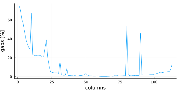
The gapfraction and coverage functions return a vector of numbers between 0.0 and 1.0 (fraction of...). Sometime it's useful to plot this data to quickly understand the MSA structure. In this example, we are going to use the Plots package for plotting, with the GR backend, but you are free to use any of the Julia plotting libraries.
using MIToS.MSA

msa = read_file(
    "https://raw.githubusercontent.com/diegozea/MIToS.jl/master/docs/data/PF18883.stockholm.gz",
    Stockholm,
)

using Plots

gr(size = (600, 300))

plot(
    # x is a range from 1 to the number of columns
    1:ncolumns(msa),
    # y is a Vector{Float64} with the percentage of gaps of each column
    vec(columngapfraction(msa)) .* 100.0,
    linetype = :line,
    ylabel = "gaps [%]",
    xlabel = "columns",
    legend = false,
)
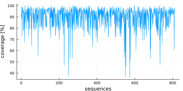
plot(
    # x is a range from 1 to the number of sequences
    1:nsequences(msa),
    # y is a Vector{Float64} with the coverage of each sequence
    vec(coverage(msa)) .* 100,
    linetype = :line,
    ylabel = "coverage [%]",
    xlabel = "sequences",
    legend = false,
)
plot(msa)
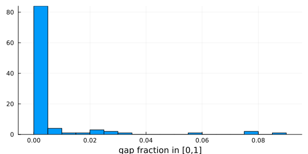
Example: Filter sequences per coverage and columns per gap fraction
Taking advantage of the filter...! functions and the coverage and columngapfraction functions, it's possible to delete short sequences or columns with a lot of gaps.
println("\tsequences\tcolumns")
println("Before:\t", nsequences(msa), "\t\t", ncolumns(msa))
# delete sequences with less than 90% coverage of the MSA length:
filtersequences!(msa, coverage(msa) .>= 0.9)
# delete columns with more than 10% of gaps:
filtercolumns!(msa, columngapfraction(msa) .<= 0.1)
println("After:\t", nsequences(msa), "\t\t", ncolumns(msa))
sequences columns
Before: 859 116
After: 400 101histogram(
vec(columngapfraction(msa)),
# Using vec() to get a Vector{Float64} with the fraction of gaps of each column
xlabel = "gap fraction in [0,1]",
bins = 20,
legend = false,
)
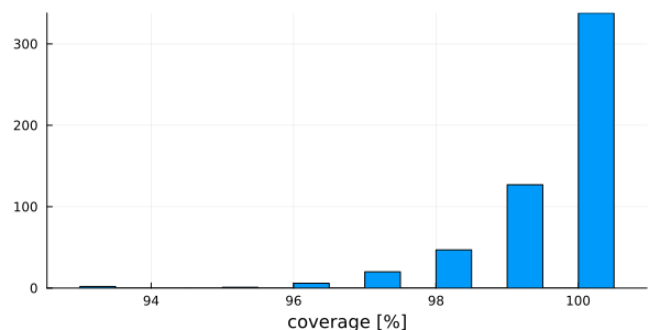
histogram(
    vec(coverage(msa) .* 100.0), #  Column with the coverage of each sequence
    xlabel = "coverage [%]",
    legend = false,
)
Example: Plotting the percentage of identity between sequences
The distribution of the percentage of identity between every pair of sequences in an MSA, gives an idea of the MSA diversity. In this example, we are using percentidentity over an MSA to get those identity values.
using MIToS.MSA
msa = read_file(
    "https://raw.githubusercontent.com/diegozea/MIToS.jl/master/docs/data/PF18883.stockholm.gz",
    Stockholm,
)
pid = percentidentity(msa)
MIToS stores the matrix of percentage of identity between the aligned sequences as a PairwiseListMatrix from the PairwiseListMatrices package. This matrix type saves RAM, allowing the storage of big matrices. In this example, we use the to_table function of PairwiseListMatrices to convert the matrix into a table with indices.
using PairwiseListMatrices

pidtable = to_table(pid, diagonal = false)
368511×3 Matrix{Any}:
"Q13FK3_PARXL/450-568" "A0A2C6C5P0_9GAMM/492-602" 35.3448
"Q13FK3_PARXL/450-568" "A0A0A7A549_SHIDY/581-689" 25.8621
"Q13FK3_PARXL/450-568" "A0A1E3VNB9_9HYPH/439-551" 31.0345
"Q13FK3_PARXL/450-568" "A0A4R0YPQ6_9GAMM/572-696" 32.7586
"Q13FK3_PARXL/450-568" "A0A1I0DBW0_9GAMM/2097-2206" 25.8621
"Q13FK3_PARXL/450-568" "A7ZLW8_ECO24/839-959" 29.3103
"Q13FK3_PARXL/450-568" "B7LGS8_ECO55/291-403" 31.8966
"Q13FK3_PARXL/450-568" "A0A840ATF5_9HYPH/823-930" 33.6207
"Q13FK3_PARXL/450-568" "D2TGE8_CITRI/464-578" 26.7241
"Q13FK3_PARXL/450-568" "A0A8T9G3H3_9HYPH/517-631" 30.1724
⋮
"A0A2T5HR93_9PSED/761-875" "M4RY98_9SPHN/2929-3041" 41.7391
"A0A2T5HR93_9PSED/761-875" "A0A2Z3I4X0_9GAMM/539-665" 32.7586
"A0A2T5HR93_9PSED/761-875" "A0A4R0YYZ7_9GAMM/486-609" 51.7241
"A0A843YVK4_9BURK/1398-1516" "M4RY98_9SPHN/2929-3041" 40.3509
"A0A843YVK4_9BURK/1398-1516" "A0A2Z3I4X0_9GAMM/539-665" 32.1739
"A0A843YVK4_9BURK/1398-1516" "A0A4R0YYZ7_9GAMM/486-609" 48.2759
"M4RY98_9SPHN/2929-3041" "A0A2Z3I4X0_9GAMM/539-665" 37.234
"M4RY98_9SPHN/2929-3041" "A0A4R0YYZ7_9GAMM/486-609" 37.5
"A0A2Z3I4X0_9GAMM/539-665" "A0A4R0YYZ7_9GAMM/486-609" 34.8214The function quantile gives a quick idea of the percentage identity distribution of the MSA.
using Statistics

quantile(convert(Vector{Float64}, pidtable[:, 3]), [0.00, 0.25, 0.50, 0.75, 1.00])
5-element Vector{Float64}:
0.9090909090909091
29.09090909090909
34.285714285714285
39.63963963963964
100.0The function meanpercentidentity gives the mean value of the percent identity distribution for MSA with less than 300 sequences, or a quick estimate (mean PID in a random sample of sequence pairs) otherwise unless you set exact to true.
meanpercentidentity(msa)34.4666889861005One can easily plot that matrix and its distribution using the heatmap and histogram functions of the Plots package.
using Plots
gr()
heatmap(convert(Matrix, pid), yflip = true, ratio = :equal)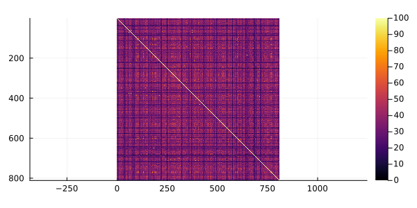
histogram(pidtable[:, 3], xlabel = "Percentage of identity", legend = false)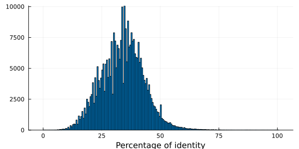
Sequence clustering
The MSA module allows to clusterize sequences in an MSA. The hobohmI function takes as input an MSA followed by an identity threshold value, and returns a Clusters type with the result of a Hobohm I sequence clustering [2]. The Hobohm I algorithm will add a sequence to an existing cluster, if the percentage of identity is equal or greater than the threshold. MSA defines the functions nelements to get the resulting number of clusters. You can access the clustersize field of the Clusters type to get the number of sequences in each cluster and the clusters to get the cluster number of each sequence. The most important method is getweight, which returns the weight of each sequence. This method is used in the Information module of MIToS to reduce redundancy. If you want, you can also use the Clusters object with the Clustering.jl package. Thanks to the package extension mechanism, if Clustering.jl is loaded, you can use functions like Clustering.nclusters, Clustering.counts, and Clustering.assignments directly on Clusters objects. Additionally, you can convert a ClusteringResult object into a Clusters object to use it with MIToS. This allows you to take advantage of the algorithms and utilities provided by Clustering.jl.
The hobohmI function can accept any vector of items, along with a custom within_cluster function as its first argument. This means you can use hobohmI to cluster not just MSAs, but any type of data—such as unaligned sequences, protein structures, or any other collection of items.
Example: Reducing redundancy of a MSA
MSAs can suffer from an unnatural sequence redundancy and a high number of protein fragments. In this example, we are using a sequence clustering to make a non-redundant set of representative sequences. We are going to use the function hobohmI to perform the clustering with the Hobohm I algorithm at 62% identity.
using MIToS.MSA
using Clustering # to use the nclusters and assignments functions

msa = read_file(
    "https://raw.githubusercontent.com/diegozea/MIToS.jl/master/docs/data/PF18883.stockholm.gz",
    Stockholm,
)

println("This MSA has ", nsequences(msa), " sequences...")
This MSA has 859 sequences...clusters = hobohmI(msa, 62)MIToS.MSA.Clusters([2, 1, 5, 1, 1, 1, 8, 2, 1, 2 … 1, 1, 1, 1, 1, 1, 1, 1, 1, 1], [1, 2, 3, 4, 5, 6, 7, 8, 9, 10 … 481, 19, 126, 482, 11, 179, 135, 16, 101, 359], [0.5, 1.0, 0.2, 1.0, 1.0, 1.0, 0.125, 0.5, 1.0, 0.5 … 1.0, 0.08333333333333333, 0.14285714285714285, 1.0, 0.027777777777777776, 0.3333333333333333, 0.25, 0.05, 0.2, 0.5])println(
"...but has only ",
nclusters(clusters),
" sequence clusters after a clustering at 62% identity.",
)...but has only 482 sequence clusters after a clustering at 62% identity.using Plots
gr()
plot(msa)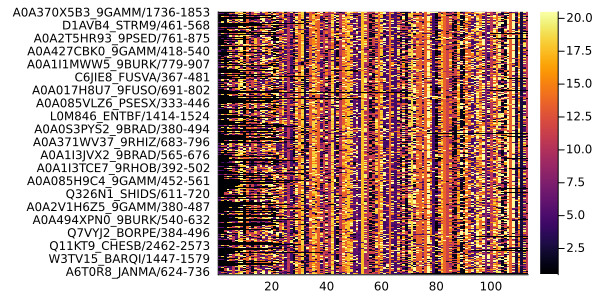
We are going to use the DataFrames package to easily select the sequence with the highest coverage of each cluster.
using DataFrames

df = DataFrame(
    seqnum = 1:nsequences(msa),
    seqname = sequencenames(msa),
    cluster = assignments(clusters), # the cluster number/index of each sequence
    coverage = vec(coverage(msa)),
)

first(df, 5)| Row | seqnum | seqname | cluster | coverage |
|---|---|---|---|---|
| Int64 | String | Int64 | Float64 | |
| 1 | 1 | Q13FK3_PARXL/450-568 | 1 | 0.991379 |
| 2 | 2 | A0A2C6C5P0_9GAMM/492-602 | 2 | 0.931034 |
| 3 | 3 | A0A0A7A549_SHIDY/581-689 | 3 | 0.87931 |
| 4 | 4 | A0A1E3VNB9_9HYPH/439-551 | 4 | 0.775862 |
| 5 | 5 | A0A4R0YPQ6_9GAMM/572-696 | 5 | 0.982759 |
It is possible to use this DataFrame and Plots to plot the sequence coverage of the MSA and also an histogram of the number of sequences in each cluster:
using StatsPlots # Plotting DataFrames
h = @df df histogram(:cluster, ylabel = "nseq")
p = @df df plot(:cluster, :coverage, linetype = :scatter)
plot(p, h, nc = 1, xlim = (0, nclusters(clusters) + 1), legend = false)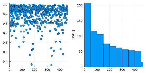
We use the Split-Apply-Combine strategy, though the groupby and combine function of the DataFrames package, to select the sequence of highest coverage for each cluster.
grouped_df = groupby(df, :cluster)

maxcoverage = combine(grouped_df) do cl
    row_index = findmax(cl.coverage)[2]
    cl[row_index, [:seqnum, :seqname, :coverage]]
end

first(maxcoverage, 5)| Row | cluster | seqnum | seqname | coverage |
|---|---|---|---|---|
| Int64 | Int64 | String | Float64 | |
| 1 | 1 | 1 | Q13FK3_PARXL/450-568 | 0.991379 |
| 2 | 2 | 2 | A0A2C6C5P0_9GAMM/492-602 | 0.931034 |
| 3 | 3 | 3 | A0A0A7A549_SHIDY/581-689 | 0.87931 |
| 4 | 4 | 4 | A0A1E3VNB9_9HYPH/439-551 | 0.775862 |
| 5 | 5 | 5 | A0A4R0YPQ6_9GAMM/572-696 | 0.982759 |
p = @df maxcoverage plot(:cluster, :coverage, linetype = :scatter)
h = @df maxcoverage histogram(:cluster, ylabel = "nseq")
plot(p, h, nc = 1, xlim = (0, nclusters(clusters) + 1), legend = false)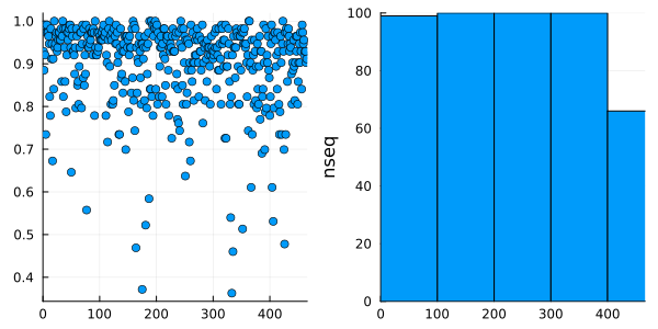
We can easily generate a mask using list comprehension, to select only the representative sequences of the MSA (deleting the rest of the sequences with filtersequences!).
cluster_references = Bool[seqnum in maxcoverage.seqnum for seqnum = 1:nsequences(msa)]859-element Vector{Bool}:
1
1
1
1
1
1
0
1
1
0
⋮
0
0
1
0
0
0
0
0
0filtersequences!(msa, cluster_references)AnnotatedMultipleSequenceAlignment with 505 annotations : 482×116 Named Matrix{MIToS.MSA.Residue}
Seq ╲ Col │ 45 46 47 48 49 … 476 477 478 479 480
───────────────────────────┼────────────────────────────────────────────────────
Q13FK3_PARXL/450-568 │ S T A T N … F D Y L L
A0A2C6C5P0_9GAMM/492-602 │ - - L T G F D Y F L
A0A0A7A549_SHIDY/581-689 │ - - - - - Y D Y R L
A0A1E3VNB9_9HYPH/439-551 │ - - - - - F A Y G L
A0A4R0YPQ6_9GAMM/572-696 │ - K L G R W Q Y T L
A0A1I0DBW0_9GAMM/2097-2206 │ - - - - - Y D Y Q L
B7LGS8_ECO55/291-403 │ S T V S N Y E Y S L
A0A840ATF5_9HYPH/823-930 │ - - - - - Y D Y R L
⋮ ⋮ ⋮ ⋮ ⋮ ⋮ ⋱ ⋮ ⋮ ⋮ ⋮ ⋮
A0A2I0FW79_9GAMM/569-677 │ - N V D E Y E Y F L
A0A840RAU7_9NEIS/64-173 │ - - - - - L D Y R L
A0A2U8E693_9BACT/1307-1431 │ - - - - - Y E Y Q L
A0A7H0GP28_9BURK/261-378 │ - - - - - Y A Y K L
A0A6N7QQ84_9GAMM/260-379 │ - - - - - Y E Y R L
A0A6M8UER1_9GAMM/583-690 │ S S V S Q Y E Y K L
A0AAE3D2V4_9HYPH/574-688 │ - - - - - F E Y G L
A0A1E3WDC8_9HYPH/497-591 │ - - - - - … F D Y D Lplot(msa)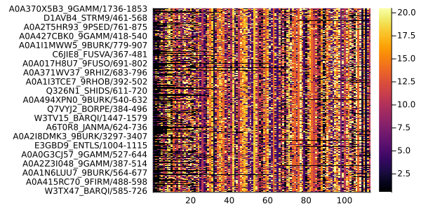
Concatenating MSAs
Concatenating multiple sequence alignments can be helpful in various bioinformatics applications. It allows researchers to combine the alignments of different sequences or regions into a single MSA for further analysis. Examples of this maneuver are concatenating two protein sequences from the same organism to estimate coevolution among those proteins or to model the protein-protein interaction using tools such as AlphaFold.
Horizontal and Vertical Concatenation
We can concatenate two MSAs as matrices using Julia's hcat and vcat functions. However, MIToS defines special methods for these functions on MSA objects to deal with sequence and column names and annotations. To use hcat, we only need the MSA having the same number of sequences. The hcat function will concatenate the first sequence of the first MSA with the first sequence of the second MSA, and so on. For example, let's define two small MSAs msa_a and msa_b, and concatenate them horizontally:
julia> using MIToS.MSAjulia> msa_a = AnnotatedMultipleSequenceAlignment(Residue[ 'A' 'R' 'N' 'D' 'C' 'Q' ]);julia> rename_sequences!(msa_a, ["SEQ1_A", "SEQ2_A"])AnnotatedMultipleSequenceAlignment with 0 annotations : 2×3 Named Matrix{MIToS.MSA.Residue} Seq ╲ Col │ 1 2 3 ──────────┼──────── SEQ1_A │ A R N SEQ2_A │ D C Qjulia> msa_b = AnnotatedMultipleSequenceAlignment(Residue[ 'N' 'Q' 'E' 'G' ]);julia> rename_sequences!(msa_b, ["SEQ1_B", "SEQ2_B"])AnnotatedMultipleSequenceAlignment with 0 annotations : 2×2 Named Matrix{MIToS.MSA.Residue} Seq ╲ Col │ 1 2 ──────────┼───── SEQ1_B │ N Q SEQ2_B │ E Gjulia> concatenated_msa = hcat(msa_a, msa_b)AnnotatedMultipleSequenceAlignment with 1 annotations : 2×5 Named Matrix{MIToS.MSA.Residue} Seq ╲ Col │ 1_1 1_2 1_3 2_1 2_2 ────────────────┼──────────────────────── SEQ1_A_&_SEQ1_B │ A R N N Q SEQ2_A_&_SEQ2_B │ D C Q E G
As you might have noticed, the hcat function preserves the sequence names by concatenating them using _&_ as a separator. So, the first sequence of the concatenated MSA is SEQ1_A_&_SEQ1_B. Also, the column names have changed in the concatenated MSA. For example, the first column of msa_a is now the first column of concatenated_msa, but its name changed from 1 to 1_1. The hcat function renames the columns so that the first number, the one before the underscore, indicates the index of the sub-MSA. The first sub-MSA in the concatenated MSA is 1, the second sub-MSA is 2, and so on. This allows you to track the origin of each column in the concatenated MSA. You can access a vector of those indices using the gethcatmapping function:
julia> gethcatmapping(concatenated_msa)5-element Vector{Int64}:
 1
 1
 1
 2
 2
If we perform multiple concatenations—i.e., if we call hcat on an MSA output of another call to hcat—the hcat function will remember the sub-MSA boundaries to continue the numeration accordingly. For example, let's create and add a third MSA:
julia> msa_c = AnnotatedMultipleSequenceAlignment(Residue[ 'A' 'H' 'A' 'H' ]);julia> rename_sequences!(msa_c, ["SEQ1_C", "SEQ2_C"])AnnotatedMultipleSequenceAlignment with 0 annotations : 2×2 Named Matrix{MIToS.MSA.Residue} Seq ╲ Col │ 1 2 ──────────┼───── SEQ1_C │ A H SEQ2_C │ A Hjulia> hcat(concatenated_msa, msa_c)AnnotatedMultipleSequenceAlignment with 1 annotations : 2×7 Named Matrix{MIToS.MSA.Residue} Seq ╲ Col │ 1_1 1_2 1_3 2_1 2_2 3_1 3_2 ─────────────────────────┼────────────────────────────────── SEQ1_A_&_SEQ1_B_&_SEQ1_C │ A R N N Q A H SEQ2_A_&_SEQ2_B_&_SEQ2_C │ D C Q E G A H
As you can see, the hcat function detects the previous concatenation and continues the indexing from the last MSA. So that column 1 of msa_c is now 3_1 in the concatenated MSA. The hcat function can take more than two MSAs as arguments. For example, you can get the same result as above by calling hcat(msa_a, msa_b, msa_c).
To concatenate MSAs vertically, you can use the vcat function. The only requirement is that the MSAs have the same number of columns. For example, let's define two small MSAs. The first column of msa_a will be concatenated with the first column of msa_b, and so on:
julia> using MIToS.MSAjulia> msa_a = AnnotatedMultipleSequenceAlignment(Residue[ 'A' 'R' 'D' 'C' 'E' 'G' ])AnnotatedMultipleSequenceAlignment with 0 annotations : 3×2 Named Matrix{MIToS.MSA.Residue} Seq ╲ Col │ 1 2 ──────────┼───── 1 │ A R 2 │ D C 3 │ E Gjulia> msa_b = AnnotatedMultipleSequenceAlignment(Residue[ 'N' 'Q' 'D' 'R' ])AnnotatedMultipleSequenceAlignment with 0 annotations : 2×2 Named Matrix{MIToS.MSA.Residue} Seq ╲ Col │ 1 2 ──────────┼───── 1 │ N Q 2 │ D Rjulia> concatenated_msa = vcat(msa_a, msa_b)AnnotatedMultipleSequenceAlignment with 0 annotations : 5×2 Named Matrix{MIToS.MSA.Residue} Seq ╲ Col │ 1 2 ──────────┼───── 1_1 │ A R 1_2 │ D C 1_3 │ E G 2_1 │ N Q 2_2 │ D R
In this case, vcat adds the MSA index prefix to the sequence names. So, the sequence 1 of msa_a is now 1_1 in the concatenated MSA. The vcat function, similar to hcat, can take more than two MSAs as arguments in case you need to concatenate multiple alignments vertically.
Joining MSAs
Sometimes, you may need to join or merge two MSAs, having different number of sequences or columns. For such cases, MIToS provides the join_msas function. This function allows you to join two MSAs based on specified matching positions or names. It supports different types of joins: inner, outer, left, and right. You can indicate the positions or names to match using an iterable of pairs or separate lists of positions or names. For example, using a vector of Pair objects, you can identify which positions on the first MSA (the first element of the pair) should match with which positions on the second MSA (the second element of the pair). Let's see that in one fictional example:
julia> using MIToS.MSAjulia> msa_a = AnnotatedMultipleSequenceAlignment(Residue[ 'A' 'R' 'D' 'G' 'K' 'E' 'G' 'R' 'D' ]);julia> rename_sequences!(msa_a, ["aa_HUMAN", "bb_MOUSE", "cc_YEAST"])AnnotatedMultipleSequenceAlignment with 0 annotations : 3×3 Named Matrix{MIToS.MSA.Residue} Seq ╲ Col │ 1 2 3 ──────────┼──────── aa_HUMAN │ A R D bb_MOUSE │ G K E cc_YEAST │ G R Djulia> msa_b = AnnotatedMultipleSequenceAlignment(Residue[ 'N' 'A' 'E' 'G' 'E' 'A' ]);julia> rename_sequences!(msa_b, ["AA_HUMAN", "BB_MOUSE", "CC_SHEEP"])AnnotatedMultipleSequenceAlignment with 0 annotations : 3×2 Named Matrix{MIToS.MSA.Residue} Seq ╲ Col │ 1 2 ──────────┼───── AA_HUMAN │ N A BB_MOUSE │ E G CC_SHEEP │ E Ajulia> pairing = ["aa_HUMAN" => "AA_HUMAN", "bb_MOUSE" => "BB_MOUSE"]2-element Vector{Pair{String, String}}: "aa_HUMAN" => "AA_HUMAN" "bb_MOUSE" => "BB_MOUSE"julia> join_msas(msa_a, msa_b, pairing)AnnotatedMultipleSequenceAlignment with 2 annotations : 4×5 Named Matrix{MIToS.MSA.Residue} Seq ╲ Col │ 1_1 1_2 1_3 2_1 2_2 ────────────────────┼──────────────────────── aa_HUMAN_&_AA_HUMAN │ A R D N A bb_MOUSE_&_BB_MOUSE │ G K E E G cc_YEAST │ G R D - - CC_SHEEP │ - - - E A
As we can see, the join_msas function has matched the sequences on both MSAs based on the specified pairing—in this example, we create a dictionary to pair the sequences from the same species. The join_msas have two important keyword arguments: kind and axis. By default, the function performs an outer join (kind = :outer) and matches the sequences (axis = 1). You can change these arguments to perform other kinds of joins or to match the columns. Since we performed an outer join, the resulting MSA contains all sequences from both input MSAs, and join_msas have added gaps where the sequences do not match.