Information

Extracting evolutionary signals, such as conservation and coevolution, from Multiple Sequence Alignments (MSAs) is a common task in bioinformatics. There are several methods to estimate these signals, including information measures like Shannon Entropy—to assess the conservation of a position—and Mutual Information—to assess the coevolution between two positions. The Information module of MIToS defines types and functions useful for calculating those information measures over an MSA. This module was designed to count Residues (defined in the MSA module) in special contingency tables (as fast as possible) and to derive probabilities from these counts. It also includes methods for applying corrections to those tables, e.g., pseudo counts and pseudo frequencies. Finally, Information allows using probabilities and counts to estimate information measures and other frequency-based values.

using MIToS.Information # to load the Information module

Features

Estimate multi-dimensional frequencies (counts) and probability tables from sequences, MSA columns, etc...
Corrections for a small number of observations
Corrections for data redundancy on an MSA
Estimate information measures such as Shannon entropy, mutual information, etc...
Calculate corrected mutual information between residues

Information

Counting residues

You can use the frequencies and probabilities functions to easily calculate the amino acid frequencies or probabilities of a sequence or a column of an MSA. The number of sequences/columns determines the dimension of the resulting table. Let's see an example using the frequencies function to calculate the frequencies of each pair of residues in two columns of an MSA. The resulting Frequencies object contains the bidimensional contingency table, the marginal values, and the total.

using MIToS.Information
using MIToS.MSA # to use res"..." to create Vector{Residue}

column_i = res"AARANHDDRDC-"
column_j = res"-ARRNHADRAVY"
#   Nij[R,R] =   1     1   = 2

Nij = frequencies(column_i, column_j)

MIToS.Information.Frequencies{Float64, 2, MIToS.MSA.UngappedAlphabet} wrapping a MIToS.Information.ContingencyTable{Float64, 2, MIToS.MSA.UngappedAlphabet} : 

table : 20×20 Named Matrix{Float64}
Dim_1 ╲ Dim_2 │   A    R    N    D    C    Q  …    P    S    T    W    Y    V
──────────────┼──────────────────────────────────────────────────────────────
A             │ 1.0  1.0  0.0  0.0  0.0  0.0  …  0.0  0.0  0.0  0.0  0.0  0.0
R             │ 0.0  2.0  0.0  0.0  0.0  0.0     0.0  0.0  0.0  0.0  0.0  0.0
N             │ 0.0  0.0  1.0  0.0  0.0  0.0     0.0  0.0  0.0  0.0  0.0  0.0
D             │ 2.0  0.0  0.0  1.0  0.0  0.0     0.0  0.0  0.0  0.0  0.0  0.0
C             │ 0.0  0.0  0.0  0.0  0.0  0.0     0.0  0.0  0.0  0.0  0.0  1.0
Q             │ 0.0  0.0  0.0  0.0  0.0  0.0     0.0  0.0  0.0  0.0  0.0  0.0
E             │ 0.0  0.0  0.0  0.0  0.0  0.0     0.0  0.0  0.0  0.0  0.0  0.0
G             │ 0.0  0.0  0.0  0.0  0.0  0.0     0.0  0.0  0.0  0.0  0.0  0.0
⋮                 ⋮    ⋮    ⋮    ⋮    ⋮    ⋮  ⋱    ⋮    ⋮    ⋮    ⋮    ⋮    ⋮
M             │ 0.0  0.0  0.0  0.0  0.0  0.0     0.0  0.0  0.0  0.0  0.0  0.0
F             │ 0.0  0.0  0.0  0.0  0.0  0.0     0.0  0.0  0.0  0.0  0.0  0.0
P             │ 0.0  0.0  0.0  0.0  0.0  0.0     0.0  0.0  0.0  0.0  0.0  0.0
S             │ 0.0  0.0  0.0  0.0  0.0  0.0     0.0  0.0  0.0  0.0  0.0  0.0
T             │ 0.0  0.0  0.0  0.0  0.0  0.0     0.0  0.0  0.0  0.0  0.0  0.0
W             │ 0.0  0.0  0.0  0.0  0.0  0.0     0.0  0.0  0.0  0.0  0.0  0.0
Y             │ 0.0  0.0  0.0  0.0  0.0  0.0     0.0  0.0  0.0  0.0  0.0  0.0
V             │ 0.0  0.0  0.0  0.0  0.0  0.0  …  0.0  0.0  0.0  0.0  0.0  0.0

marginals : 20×2 Named Matrix{Float64}
Residue ╲ Dim │ Dim_1  Dim_2
──────────────┼─────────────
A             │   2.0    3.0
R             │   2.0    3.0
N             │   1.0    1.0
D             │   3.0    1.0
C             │   1.0    0.0
Q             │   0.0    0.0
E             │   0.0    0.0
G             │   0.0    0.0
⋮                   ⋮      ⋮
M             │   0.0    0.0
F             │   0.0    0.0
P             │   0.0    0.0
S             │   0.0    0.0
T             │   0.0    0.0
W             │   0.0    0.0
Y             │   0.0    0.0
V             │   0.0    1.0

total : 10.0

You can use sum to get the stored total:

sum(Nij)

10.0

Here, the total is 10.0, because there are 12 residues on each column, but 2 are gaps. Since the default alphabet used by frequency is UngappedAlphabet(), the gaps are not counted.

Contingency tables can be indexed using Int (the coordinates in the table) or Residues. For example, to get the number of times an arginine (R) is found in the same sequence in both columns, you can use:

Nij[Residue('R'), Residue('R')]

2.0

Or, since the arginine is in the second row and the second column of the table—this is because the arginine is the second residue in the UngappedAlphabet()—you can use:

Nij[2, 2]

2.0

Indexing with `Int`

The index refers to the specific position in the table, e.g., [2,2] references the second row and the second column. For GappedAlphabet() and UngappedAlphabet(), the index is the same as the position of the residue in the alphabet. However, for ReducedAlphabet(), the index will be the number of the group to which the residue belongs. For example, if the alphabet is ReducedAlphabet("(AILMV)(NQST)(RHK)(DE)(FWY)CGP"), the index of the arginine (R) will be 3 rather than 2. Therefore, it is recommended that you use a Residue object to index the table to avoid subtle bugs if the alphabet changes.

You can change the alphabet used to count residues by setting the alphabet keyword of the frequencies function. Let's see an example with an reduced alphabet:

using MIToS.Information
using MIToS.MSA

alphabet = ReducedAlphabet("(AILMV)(NQST)(RHK)(DE)(FWY)CGP")

column_i = res"AARANHDDRDC-"
column_j = res"-ARRNHADRAVY"
#   Fij[R,R] =   1  1  1   = 3 # RHK

Fij = frequencies(column_i, column_j, alphabet = alphabet)

MIToS.Information.Frequencies{Float64, 2, MIToS.MSA.ReducedAlphabet} wrapping a MIToS.Information.ContingencyTable{Float64, 2, MIToS.MSA.ReducedAlphabet} : 

table : 8×8 Named Matrix{Float64}
Dim_1 ╲ Dim_2 │ AILMV   NQST    RHK     DE    FWY      C      G      P
──────────────┼───────────────────────────────────────────────────────
AILMV         │   1.0    0.0    1.0    0.0    0.0    0.0    0.0    0.0
NQST          │   0.0    1.0    0.0    0.0    0.0    0.0    0.0    0.0
RHK           │   0.0    0.0    3.0    0.0    0.0    0.0    0.0    0.0
DE            │   2.0    0.0    0.0    1.0    0.0    0.0    0.0    0.0
FWY           │   0.0    0.0    0.0    0.0    0.0    0.0    0.0    0.0
C             │   1.0    0.0    0.0    0.0    0.0    0.0    0.0    0.0
G             │   0.0    0.0    0.0    0.0    0.0    0.0    0.0    0.0
P             │   0.0    0.0    0.0    0.0    0.0    0.0    0.0    0.0

marginals : 8×2 Named Matrix{Float64}
Residue ╲ Dim │ Dim_1  Dim_2
──────────────┼─────────────
AILMV         │   2.0    4.0
NQST          │   1.0    1.0
RHK           │   3.0    4.0
DE            │   3.0    1.0
FWY           │   0.0    0.0
C             │   1.0    0.0
G             │   0.0    0.0
P             │   0.0    0.0

total : 10.0

Fij[Residue('R'), Residue('R')]

3.0

Example: Plotting the probabilities of each residue in a sequence

Like the frequencies function, the probabilities function can take at least one sequence or column (a vector of Residue objects) and return the probabilities of each residue. Optionally, as before, the keyword argument alphabet could be used to count some residues in the same table cell.

probabilities(res"AARANHDDRDC", alphabet = alphabet)

MIToS.Information.Probabilities{Float64, 1, MIToS.MSA.ReducedAlphabet} wrapping a MIToS.Information.ContingencyTable{Float64, 1, MIToS.MSA.ReducedAlphabet} : 

table : 8-element Named Vector{Float64}
Dim_1  │ 
───────┼──────────
AILMV  │  0.272727
NQST   │ 0.0909091
RHK    │  0.272727
DE     │  0.272727
FWY    │       0.0
C      │ 0.0909091
G      │       0.0
P      │       0.0

total : 1.0

Here, we are going to use the probabilities function to get the residue probabilities of a particular sequence from UniProt.

julia> using MIToS.Information
julia> using MIToS.MSA
julia> file_name = "http://www.uniprot.org/uniprot/P29374.fasta""http://www.uniprot.org/uniprot/P29374.fasta"
julia> sequences = read_file(file_name, FASTASequences)1-element Vector{MIToS.MSA.AnnotatedSequence}:
 [M K … C R]
julia> Pa = probabilities(sequences[1])MIToS.Information.Probabilities{Float64, 1, MIToS.MSA.UngappedAlphabet} wrapping a MIToS.Information.ContingencyTable{Float64, 1, MIToS.MSA.UngappedAlphabet} :

table : 20-element Named Vector{Float64}
Dim_1  │
───────┼───────────
A      │   0.043755
R      │  0.0517104
N      │  0.0469372
D      │  0.0755768
C      │  0.0135243
Q      │   0.035004
E      │   0.134447
G      │   0.043755
⋮                 ⋮
M      │  0.0159109
F      │  0.0190931
P      │  0.0445505
S      │   0.100239
T      │  0.0493238
W      │ 0.00636436
Y      │  0.0198886
V      │  0.0517104

total : 1.0

using Plots # We choose Plots because it's intuitive and concise
gr(size = (600, 300))

Plots.GRBackend()

You can plot together with the probabilities of each residue in a given sequence, the probabilities of each residue estimated with the BLOSUM62 substitution matrix. That matrix is exported as a constant by the Information module as BLOSUM62_Pi.

bar(1:20, [Pa BLOSUM62_Pi], lab = ["Sequence" "BLOSUM62"], alpha = 0.5)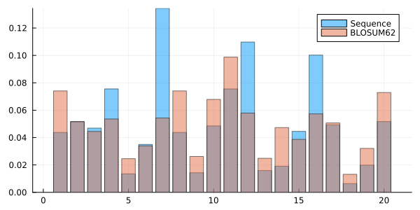

Low-level interface

You can work directly with the ContingencyTable type if you want performance. The MIToS Information module also defines two types wrapping this multi-dimensional array; Frequencies and Probabilities, to store occurrences or probabilities, respectively. The ContingencyTable type stores the contingency matrix, its marginal values, and its total. These three types are parametric, taking three ordered parameters:

T: The type used for storing the counts or probabilities, e.g., Float64. If more precision is needed, BigFloat is possible.
N: It's the dimension of the table and should be an Int.
A: This should be a type, subtype of ResidueAlphabet, i.e.: UngappedAlphabet, GappedAlphabet, or ReducedAlphabet.

Note

ContingencyTable can be used to store probabilities or counts. The wrapper types Probabilities and Frequencies are mainly intended to dispatch in methods that need to know if the matrix has probabilities or counts. For example, the implementation of shannon_entropy is faster when the table is a Frequencies object.

In this way, a matrix for storing pairwise probabilities of residues (without gaps) can be initialized using:

using MIToS.Information

Pij = ContingencyTable(Float64, Val{2}, UngappedAlphabet())

MIToS.Information.ContingencyTable{Float64, 2, MIToS.MSA.UngappedAlphabet} : 

table : 20×20 Named Matrix{Float64}
Dim_1 ╲ Dim_2 │   A    R    N    D    C    Q  …    P    S    T    W    Y    V
──────────────┼──────────────────────────────────────────────────────────────
A             │ 0.0  0.0  0.0  0.0  0.0  0.0  …  0.0  0.0  0.0  0.0  0.0  0.0
R             │ 0.0  0.0  0.0  0.0  0.0  0.0     0.0  0.0  0.0  0.0  0.0  0.0
N             │ 0.0  0.0  0.0  0.0  0.0  0.0     0.0  0.0  0.0  0.0  0.0  0.0
D             │ 0.0  0.0  0.0  0.0  0.0  0.0     0.0  0.0  0.0  0.0  0.0  0.0
C             │ 0.0  0.0  0.0  0.0  0.0  0.0     0.0  0.0  0.0  0.0  0.0  0.0
Q             │ 0.0  0.0  0.0  0.0  0.0  0.0     0.0  0.0  0.0  0.0  0.0  0.0
E             │ 0.0  0.0  0.0  0.0  0.0  0.0     0.0  0.0  0.0  0.0  0.0  0.0
G             │ 0.0  0.0  0.0  0.0  0.0  0.0     0.0  0.0  0.0  0.0  0.0  0.0
⋮                 ⋮    ⋮    ⋮    ⋮    ⋮    ⋮  ⋱    ⋮    ⋮    ⋮    ⋮    ⋮    ⋮
M             │ 0.0  0.0  0.0  0.0  0.0  0.0     0.0  0.0  0.0  0.0  0.0  0.0
F             │ 0.0  0.0  0.0  0.0  0.0  0.0     0.0  0.0  0.0  0.0  0.0  0.0
P             │ 0.0  0.0  0.0  0.0  0.0  0.0     0.0  0.0  0.0  0.0  0.0  0.0
S             │ 0.0  0.0  0.0  0.0  0.0  0.0     0.0  0.0  0.0  0.0  0.0  0.0
T             │ 0.0  0.0  0.0  0.0  0.0  0.0     0.0  0.0  0.0  0.0  0.0  0.0
W             │ 0.0  0.0  0.0  0.0  0.0  0.0     0.0  0.0  0.0  0.0  0.0  0.0
Y             │ 0.0  0.0  0.0  0.0  0.0  0.0     0.0  0.0  0.0  0.0  0.0  0.0
V             │ 0.0  0.0  0.0  0.0  0.0  0.0  …  0.0  0.0  0.0  0.0  0.0  0.0

marginals : 20×2 Named Matrix{Float64}
Residue ╲ Dim │ Dim_1  Dim_2
──────────────┼─────────────
A             │   0.0    0.0
R             │   0.0    0.0
N             │   0.0    0.0
D             │   0.0    0.0
C             │   0.0    0.0
Q             │   0.0    0.0
E             │   0.0    0.0
G             │   0.0    0.0
⋮                   ⋮      ⋮
M             │   0.0    0.0
F             │   0.0    0.0
P             │   0.0    0.0
S             │   0.0    0.0
T             │   0.0    0.0
W             │   0.0    0.0
Y             │   0.0    0.0
V             │   0.0    0.0

total : 0.0

Note that the dimension of the table is indicated using Val{2} rather than 2, so that Julia knows that the table is two-dimensional at compile time.

You can also obtain the ContingencyTable wrapped in a Frequencies object using the getcontingencytable function. For example, you can take a table of counts and normalize it using the normalize function to get a table of probabilities that you can later wrap in a Probabilities object:

using MIToS.MSA
using MIToS.Information
column_i = res"AARANHDDRDC-"
column_j = res"-ARRNHADRAVY"
Fij = frequencies(column_i, column_j)
Pij = Probabilities(normalize(getcontingencytable(Fij)))

MIToS.Information.Probabilities{Float64, 2, MIToS.MSA.UngappedAlphabet} wrapping a MIToS.Information.ContingencyTable{Float64, 2, MIToS.MSA.UngappedAlphabet} : 

table : 20×20 Named Matrix{Float64}
Dim_1 ╲ Dim_2 │   A    R    N    D    C    Q  …    P    S    T    W    Y    V
──────────────┼──────────────────────────────────────────────────────────────
A             │ 0.1  0.1  0.0  0.0  0.0  0.0  …  0.0  0.0  0.0  0.0  0.0  0.0
R             │ 0.0  0.2  0.0  0.0  0.0  0.0     0.0  0.0  0.0  0.0  0.0  0.0
N             │ 0.0  0.0  0.1  0.0  0.0  0.0     0.0  0.0  0.0  0.0  0.0  0.0
D             │ 0.2  0.0  0.0  0.1  0.0  0.0     0.0  0.0  0.0  0.0  0.0  0.0
C             │ 0.0  0.0  0.0  0.0  0.0  0.0     0.0  0.0  0.0  0.0  0.0  0.1
Q             │ 0.0  0.0  0.0  0.0  0.0  0.0     0.0  0.0  0.0  0.0  0.0  0.0
E             │ 0.0  0.0  0.0  0.0  0.0  0.0     0.0  0.0  0.0  0.0  0.0  0.0
G             │ 0.0  0.0  0.0  0.0  0.0  0.0     0.0  0.0  0.0  0.0  0.0  0.0
⋮                 ⋮    ⋮    ⋮    ⋮    ⋮    ⋮  ⋱    ⋮    ⋮    ⋮    ⋮    ⋮    ⋮
M             │ 0.0  0.0  0.0  0.0  0.0  0.0     0.0  0.0  0.0  0.0  0.0  0.0
F             │ 0.0  0.0  0.0  0.0  0.0  0.0     0.0  0.0  0.0  0.0  0.0  0.0
P             │ 0.0  0.0  0.0  0.0  0.0  0.0     0.0  0.0  0.0  0.0  0.0  0.0
S             │ 0.0  0.0  0.0  0.0  0.0  0.0     0.0  0.0  0.0  0.0  0.0  0.0
T             │ 0.0  0.0  0.0  0.0  0.0  0.0     0.0  0.0  0.0  0.0  0.0  0.0
W             │ 0.0  0.0  0.0  0.0  0.0  0.0     0.0  0.0  0.0  0.0  0.0  0.0
Y             │ 0.0  0.0  0.0  0.0  0.0  0.0     0.0  0.0  0.0  0.0  0.0  0.0
V             │ 0.0  0.0  0.0  0.0  0.0  0.0  …  0.0  0.0  0.0  0.0  0.0  0.0

marginals : 20×2 Named Matrix{Float64}
Residue ╲ Dim │ Dim_1  Dim_2
──────────────┼─────────────
A             │   0.2    0.3
R             │   0.2    0.3
N             │   0.1    0.1
D             │   0.3    0.1
C             │   0.1    0.0
Q             │   0.0    0.0
E             │   0.0    0.0
G             │   0.0    0.0
⋮                   ⋮      ⋮
M             │   0.0    0.0
F             │   0.0    0.0
P             │   0.0    0.0
S             │   0.0    0.0
T             │   0.0    0.0
W             │   0.0    0.0
Y             │   0.0    0.0
V             │   0.0    0.1

total : 1.0

Low count corrections

A low number of observations can lead to sparse contingency tables that lead to wrong probability estimations. It is shown in Buslje et al. [3] that low-count corrections, can lead to improvements in the contact prediction capabilities of the mutual information. The Information module has available two low-count corrections:

AdditiveSmoothing: Additive smoothing corrects the frequencies by adding a constant value to each cell of the table. It can be used to represent the constant value pseudocount described in Buslje et al. [3]. For example: AdditiveSmoothing(1.0) can be used to add 1.0 to each cell of the table.
BLOSUM_Pseudofrequencies: BLOSUM62-based pseudo frequencies for residues pairs, similar to Altschul et al. [4] and described in [1]

The frequencies and probabilities functions have a pseudocounts keyword argument that can take an AdditiveSmoothing value to calculate occurrences and probabilities with pseudo counts.

using MIToS.MSA
using MIToS.Information
seq = res"AAAVRNHDDRDCPPPGGPPG"
frequencies(seq, pseudocounts = AdditiveSmoothing(1.0))

MIToS.Information.Frequencies{Float64, 1, MIToS.MSA.UngappedAlphabet} wrapping a MIToS.Information.ContingencyTable{Float64, 1, MIToS.MSA.UngappedAlphabet} : 

table : 20-element Named Vector{Float64}
Dim_1  │ 
───────┼────
A      │ 4.0
R      │ 3.0
N      │ 2.0
D      │ 4.0
C      │ 2.0
Q      │ 1.0
E      │ 1.0
G      │ 4.0
⋮          ⋮
M      │ 1.0
F      │ 1.0
P      │ 6.0
S      │ 1.0
T      │ 1.0
W      │ 1.0
Y      │ 1.0
V      │ 2.0

total : 40.0

The probabilities function can also take a pseudofrequencies keyword argument that can take a BLOSUM_Pseudofrequencies object to calculate probabilities with pseudo frequencies. Note that these pseudofrequencies can only be used on bidimensional tables, i.e. passing only two sequences or columns to the probabilities function, and using UngappedAlphabet() (the default alphabet).

using MIToS.MSA
using MIToS.Information
column_i = res"ARANHDDRDC"
column_j = res"-RRNHADRAV"
probabilities(column_i, column_j, pseudofrequencies = BLOSUM_Pseudofrequencies(10, 8.512))

MIToS.Information.Probabilities{Float64, 2, MIToS.MSA.UngappedAlphabet} wrapping a MIToS.Information.ContingencyTable{Float64, 2, MIToS.MSA.UngappedAlphabet} : 

table : 20×20 Named Matrix{Float64}
Dim_1 ╲ Dim_2 │           A            R  …            Y            V
──────────────┼──────────────────────────────────────────────────────
A             │   0.0025812    0.0671681  …  0.000659565   0.00194086
R             │  0.00284631     0.133119     0.000898756   0.00172866
N             │  0.00328919   0.00301308     0.000682269   0.00145771
D             │    0.133185   0.00378038      0.00121515   0.00381553
C             │  0.00208857   0.00127052     0.000589305    0.0668084
Q             │  0.00142694   0.00247813      0.00033108  0.000699949
E             │    0.003512   0.00324315     0.000557825   0.00134036
G             │  0.00214771   0.00303399     0.000436419   0.00119478
⋮                         ⋮            ⋮  ⋱            ⋮            ⋮
M             │ 0.000521219  0.000978248     0.000135993  0.000411015
F             │ 0.000778701   0.00119943     0.000210395  0.000551961
P             │  0.00101033   0.00142181     0.000203036  0.000567906
S             │  0.00244132   0.00361921     0.000499758   0.00141208
T             │  0.00169218   0.00249277     0.000346269   0.00108457
W             │ 0.000196949  0.000349704      5.40184e-5  0.000128953
Y             │ 0.000675454   0.00115816     0.000266102  0.000431768
V             │  0.00138077   0.00259873  …   0.00032221   0.00125388

marginals : 20×2 Named Matrix{Float64}
Residue ╲ Dim │      Dim_1       Dim_2
──────────────┼───────────────────────
A             │   0.093333    0.166519
R             │    0.16693    0.243387
N             │  0.0956191   0.0918704
D             │   0.252676   0.0952168
C             │  0.0886361  0.00561482
Q             │  0.0151327   0.0160779
E             │  0.0275049   0.0232662
G             │  0.0214472   0.0219686
⋮                        ⋮           ⋮
M             │ 0.00609007  0.00760737
F             │ 0.00868029  0.00993714
P             │ 0.00977333   0.0100034
S             │  0.0246863   0.0255755
T             │  0.0172989   0.0186683
W             │ 0.00226332  0.00252896
Y             │ 0.00874174  0.00980948
V             │  0.0158639   0.0893325

total : 1.0

Low-level interface

If you have a preallocated ContingencyTable, for performance reasons, you can use frequencies! or the probabilities! functions to fill it. That prevents the creation of a new table as frequencies and probabilities do. However, you should note that frequencies! and probabilities! add the new counts to the pre-existing values. Therefore, you can use the cleanup! function to set the table to zero before filling it.

Let's see an example, in this case we start with a table of zeros, Nij, and fill it with the counts of the residues in the columns column_i and column_j using the frequencies! function. Since we start with a new table, we don't need to use cleanup!.

using MIToS.MSA
using MIToS.Information

file_name = "https://raw.githubusercontent.com/diegozea/MIToS.jl/master/docs/data/PF18883.stockholm.gz"

msa = read_file(file_name, Stockholm)

column_i = msa[:, 1]
column_j = msa[:, 2]

const ALPHABET = ReducedAlphabet("(AILMV)(NQST)(RHK)(DE)(FWY)CGP")

Nij = ContingencyTable(Float64, Val{2}, ALPHABET)

frequencies!(Nij, column_i, column_j)

MIToS.Information.ContingencyTable{Float64, 2, MIToS.MSA.ReducedAlphabet} : 

table : 8×8 Named Matrix{Float64}
Dim_1 ╲ Dim_2 │ AILMV   NQST    RHK     DE    FWY      C      G      P
──────────────┼───────────────────────────────────────────────────────
AILMV         │   0.0    0.0    0.0    0.0    0.0    0.0    0.0    0.0
NQST          │  42.0  114.0   10.0   33.0    1.0    1.0    0.0    0.0
RHK           │   0.0    0.0    0.0    0.0    0.0    0.0    0.0    0.0
DE            │   0.0    0.0    0.0    0.0    0.0    0.0    0.0    0.0
FWY           │   0.0    0.0    0.0    0.0    0.0    0.0    0.0    0.0
C             │   0.0    0.0    0.0    0.0    0.0    0.0    0.0    0.0
G             │   0.0    0.0    0.0    0.0    0.0    0.0    0.0    0.0
P             │   0.0    0.0    0.0    0.0    0.0    0.0    0.0    0.0

marginals : 8×2 Named Matrix{Float64}
Residue ╲ Dim │ Dim_1  Dim_2
──────────────┼─────────────
AILMV         │   0.0   42.0
NQST          │ 201.0  114.0
RHK           │   0.0   10.0
DE            │   0.0   33.0
FWY           │   0.0    1.0
C             │   0.0    1.0
G             │   0.0    0.0
P             │   0.0    0.0

total : 201.0

In cases like the above, where there are few observations, applying a constant pseudocount to the contingency table could be beneficial. This module defines the type AdditiveSmoothing and the corresponding fill! and apply_pseudocount! methods to efficiently fill or add a constant value to each element of the table.

apply_pseudocount!(Nij, AdditiveSmoothing(1.0))

MIToS.Information.ContingencyTable{Float64, 2, MIToS.MSA.ReducedAlphabet} : 

table : 8×8 Named Matrix{Float64}
Dim_1 ╲ Dim_2 │ AILMV   NQST    RHK     DE    FWY      C      G      P
──────────────┼───────────────────────────────────────────────────────
AILMV         │   1.0    1.0    1.0    1.0    1.0    1.0    1.0    1.0
NQST          │  43.0  115.0   11.0   34.0    2.0    2.0    1.0    1.0
RHK           │   1.0    1.0    1.0    1.0    1.0    1.0    1.0    1.0
DE            │   1.0    1.0    1.0    1.0    1.0    1.0    1.0    1.0
FWY           │   1.0    1.0    1.0    1.0    1.0    1.0    1.0    1.0
C             │   1.0    1.0    1.0    1.0    1.0    1.0    1.0    1.0
G             │   1.0    1.0    1.0    1.0    1.0    1.0    1.0    1.0
P             │   1.0    1.0    1.0    1.0    1.0    1.0    1.0    1.0

marginals : 8×2 Named Matrix{Float64}
Residue ╲ Dim │ Dim_1  Dim_2
──────────────┼─────────────
AILMV         │   8.0   50.0
NQST          │ 209.0  122.0
RHK           │   8.0   18.0
DE            │   8.0   41.0
FWY           │   8.0    9.0
C             │   8.0    9.0
G             │   8.0    8.0
P             │   8.0    8.0

total : 265.0

If we work with a normalized contingency table or a Probabilities object and use the UnappedAlphabet(), we can apply the BLOSUM62-based pseudo frequencies to the table. For that, we can use the BLOSUM_Pseudofrequencies type and the apply_pseudofrequencies! function. That function first needs to calculate the actual probabilities $p_{a,b}$ for each pair of residues $a$, $b$. Then, it uses the conditional probability matrix BLOSUM62_Pij and the observed probabilities to calculate pseudo frequencies $G$.

\[G_{ab} = \sum_{cd} p_{cd} \cdot BLOSUM62( a | c ) \cdot BLOSUM62( b | d )\]

The apply_pseudofrequencies! function calculates the probability $P$ of each pair of residues $a$, $b$ between the columns $i$, $j$ as the weighted mean between the observed frequency $p$ and BLOSUM62-based pseudo frequency $G$. The former has α as weight, and the latter has the parameter β. We use the number of sequences or sequence clusters as α, and β is an empiric weight value that we determined to be close to 8.512.

\[P_{ab} = \frac{\alpha \cdot p_{ab} + \beta \cdot G_{ab} }{\alpha + \beta}\]

The BLOSUM_Pseudofrequencies type is defined with two parameters, α and β, that are set using the positional arguments of the constructor.

using MIToS.MSA
using MIToS.Information
column_i = res"ARANHDDRDC"
column_j = res"-RRNHADRAV"
Pij = ContingencyTable(Float64, Val{2}, UngappedAlphabet())
probabilities!(Pij, column_i, column_j)
α = 10
β = 8.512
apply_pseudofrequencies!(Pij, BLOSUM_Pseudofrequencies(α, β))

MIToS.Information.ContingencyTable{Float64, 2, MIToS.MSA.UngappedAlphabet} : 

table : 20×20 Named Matrix{Float64}
Dim_1 ╲ Dim_2 │           A            R  …            Y            V
──────────────┼──────────────────────────────────────────────────────
A             │   0.0025812    0.0671681  …  0.000659565   0.00194086
R             │  0.00284631     0.133119     0.000898756   0.00172866
N             │  0.00328919   0.00301308     0.000682269   0.00145771
D             │    0.133185   0.00378038      0.00121515   0.00381553
C             │  0.00208857   0.00127052     0.000589305    0.0668084
Q             │  0.00142694   0.00247813      0.00033108  0.000699949
E             │    0.003512   0.00324315     0.000557825   0.00134036
G             │  0.00214771   0.00303399     0.000436419   0.00119478
⋮                         ⋮            ⋮  ⋱            ⋮            ⋮
M             │ 0.000521219  0.000978248     0.000135993  0.000411015
F             │ 0.000778701   0.00119943     0.000210395  0.000551961
P             │  0.00101033   0.00142181     0.000203036  0.000567906
S             │  0.00244132   0.00361921     0.000499758   0.00141208
T             │  0.00169218   0.00249277     0.000346269   0.00108457
W             │ 0.000196949  0.000349704      5.40184e-5  0.000128953
Y             │ 0.000675454   0.00115816     0.000266102  0.000431768
V             │  0.00138077   0.00259873  …   0.00032221   0.00125388

marginals : 20×2 Named Matrix{Float64}
Residue ╲ Dim │      Dim_1       Dim_2
──────────────┼───────────────────────
A             │   0.093333    0.166519
R             │    0.16693    0.243387
N             │  0.0956191   0.0918704
D             │   0.252676   0.0952168
C             │  0.0886361  0.00561482
Q             │  0.0151327   0.0160779
E             │  0.0275049   0.0232662
G             │  0.0214472   0.0219686
⋮                        ⋮           ⋮
M             │ 0.00609007  0.00760737
F             │ 0.00868029  0.00993714
P             │ 0.00977333   0.0100034
S             │  0.0246863   0.0255755
T             │  0.0172989   0.0186683
W             │ 0.00226332  0.00252896
Y             │ 0.00874174  0.00980948
V             │  0.0158639   0.0893325

total : 1.0

Correction for data redundancy in a MSA

A simple way to reduce redundancy in an MSA without losing sequences is through clusterization and sequence weighting. The weight of each sequence should be $1/N$, where $N$ is the number of sequences in its cluster. The Clusters type of the MSA module stores the weights. This vector of weights can be extracted (with the getweight function) and used by the frequencies and probabilities functions with the keyword argument weights. Also, using the Clusters as the second argument of the function frequencies! is possible.

clusters = hobohmI(msa, 62) # from MIToS.MSA

MIToS.MSA.Clusters([1, 4, 3, 1, 2, 1, 2, 9, 9, 3  …  1, 1, 1, 1, 1, 1, 1, 1, 1, 1], [1, 2, 3, 4, 5, 6, 7, 8, 9, 10  …  297, 462, 463, 46, 122, 464, 111, 465, 429, 348], [1.0, 0.25, 0.3333333333333333, 1.0, 0.5, 1.0, 0.5, 0.1111111111111111, 0.1111111111111111, 0.3333333333333333  …  0.3333333333333333, 1.0, 1.0, 0.14285714285714285, 0.1111111111111111, 1.0, 0.3333333333333333, 1.0, 0.5, 0.3333333333333333])

frequencies(msa[:, 1], msa[:, 2], weights = clusters)

MIToS.Information.Frequencies{Float64, 2, MIToS.MSA.UngappedAlphabet} wrapping a MIToS.Information.ContingencyTable{Float64, 2, MIToS.MSA.UngappedAlphabet} : 

table : 20×20 Named Matrix{Float64}
Dim_1 ╲ Dim_2 │        A         R         N  …         W         Y         V
──────────────┼──────────────────────────────────────────────────────────────
A             │      0.0       0.0       0.0  …       0.0       0.0       0.0
R             │      0.0       0.0       0.0          0.0       0.0       0.0
N             │      0.0       0.0       0.0          0.0       0.0       0.0
D             │      0.0       0.0       0.0          0.0       0.0       0.0
C             │      0.0       0.0       0.0          0.0       0.0       0.0
Q             │      0.0       0.0       0.0          0.0       0.0       0.0
E             │      0.0       0.0       0.0          0.0       0.0       0.0
G             │      0.0       0.0       0.0          0.0       0.0       0.0
⋮                      ⋮         ⋮         ⋮  ⋱         ⋮         ⋮         ⋮
M             │      0.0       0.0       0.0          0.0       0.0       0.0
F             │      0.0       0.0       0.0          0.0       0.0       0.0
P             │      0.0       0.0       0.0          0.0       0.0       0.0
S             │  3.27778       3.2   23.1333     0.333333       0.0   12.5012
T             │      0.0       0.0       0.0          0.0       0.0       0.0
W             │      0.0       0.0       0.0          0.0       0.0       0.0
Y             │      0.0       0.0       0.0          0.0       0.0       0.0
V             │      0.0       0.0       0.0  …       0.0       0.0       0.0

marginals : 20×2 Named Matrix{Float64}
Residue ╲ Dim │    Dim_1     Dim_2
──────────────┼───────────────────
A             │      0.0   3.27778
R             │      0.0       3.2
N             │      0.0   23.1333
D             │      0.0   10.2833
C             │      0.0       1.0
Q             │      0.0      7.55
E             │      0.0    4.9619
G             │      0.0       0.0
⋮                      ⋮         ⋮
M             │      0.0       1.0
F             │      0.0       0.0
P             │      0.0       0.0
S             │  107.531   16.8833
T             │      0.0   18.4024
W             │      0.0  0.333333
Y             │      0.0       0.0
V             │      0.0   12.5012

total : 107.53055555555555

Estimating information measures on an MSA

The Information module has a number of functions defined to calculate information measures from Frequencies and Probabilities:

shannon_entropy : Shannon entropy (H)
marginal_entropy : Shannon entropy (H) of the marginals
kullback_leibler : Kullback-Leibler (KL) divergence
mutual_information : Mutual Information (MI)
normalized_mutual_information : Normalized Mutual Information (nMI) by Entropy
gap_intersection_percentage
gap_union_percentage

Information measure functions take optionally the base as a keyword argument (default: ℯ). You can set base=2 to measure information in bits.

using MIToS.Information
using MIToS.MSA

Ni = frequencies(res"PPCDPPPPPKDKKKKDDGPP") # Ni has the count table of residues in this low complexity sequence

H = shannon_entropy(Ni) # returns the Shannon entropy in nats (base e)

1.327362863420189

H = shannon_entropy(Ni, base = 2) # returns the Shannon entropy in bits (base 2)

1.9149798205164812

Information module defines special iteration functions to easily and efficiently compute a measure over a MSA. In particular, mapcolfreq! and mapseqfreq! map a function that takes a table of Frequencies or Probabilities. The table is filled in place with the counts or probabilities of each column or sequence of a MSA, respectively. mapcolpairfreq! and mapseqpairfreq! are similar, but they fill the table using pairs of columns or sequences, respectively.

This functions take three positional arguments: the function f to be calculated, the msa and table of Frequencies or Probabilities.

After that, this function takes some keyword arguments:

weights (default: NoClustering()) : Weights to be used for table counting.
pseudocounts (default: NoPseudocount()) : Pseudocount object to be applied to table.
pseudofrequencies (default: NoPseudofrequencies()) : Pseudofrequencies to be applied to the normalized (probabilities) table.
usediagonal (default: true) : Indicates if the function should be applied to pairs containing the same sequence or column.
diagonalvalue (default to zero) : The value that fills the diagonal elements of the table if usediagonal is false.

Example: Estimating H(X) and H(X, Y) over an MSA

In this example, we are going to use mapcolfreq! and mapcolpairfreq! to estimate Shannon shannon_entropy of MSA columns H(X) and the joint entropy H(X, Y) of columns pairs, respectively.

using MIToS.MSA

msa = read_file(
    "https://raw.githubusercontent.com/diegozea/MIToS.jl/master/docs/data/PF18883.stockholm.gz",
    Stockholm,
)

AnnotatedMultipleSequenceAlignment with 835 annotations : 811×113 Named Matrix{MIToS.MSA.Residue}
                 Seq ╲ Col │  53   54   55   56   57  …  428  429  430  431  432
───────────────────────────┼────────────────────────────────────────────────────
A0A370X5B3_9GAMM/1736-1853 │   -    -    -    -    -  …    Y    A    Y    R    L
D1AVB4_STRM9/461-568       │   -    -    -    -    -       Y    R    Y    R    L
A0A2T5HR93_9PSED/761-875   │   S    N    L    T    S       Y    Q    Y    T    L
A0A427CBK0_9GAMM/418-540   │   -    -    -    -    -       F    R    Y    R    L
A0A1I1MWW5_9BURK/779-907   │   -    -    -    -    -       Y    E    Y    R    L
C6JIE8_FUSVA/367-481       │   -    I    I    S    N       Y    E    Y    F    L
A0A017H8U7_9FUSO/691-802   │   S    S    V    T    E       Y    E    Y    T    L
A0A085VLZ6_PSESX/333-446   │   -    -    -    -    -       Y    E    Y    Y    L
⋮                              ⋮    ⋮    ⋮    ⋮    ⋮  ⋱    ⋮    ⋮    ⋮    ⋮    ⋮
A0A318T6N3_9RHIZ/636-751   │   -    -    -    K    T       Y    V    Y    Q    L
A0A388SGN0_9BURK/625-739   │   S    E    L    T    T       Y    L    Y    E    L
A0A443IAD3_9GAMM/1863-1969 │   -    -    -    -    -       Y    D    Y    S    L
A0A2S8VQP6_9CAUL/182-287   │   -    -    -    -    R       V    R    Y    R    -
A0A1A9RWJ5_9NEIS/1004-1099 │   S    T    V    T    N       -    -    -    -    -
A6T0K2_JANMA/343-459       │   -    -    -    -    -       Y    A    Y    T    L
Q2KVL9_BORA1/480-598       │   S    R    I    T    R       Y    E    Y    R    L
A0A2W4CX06_9RHIZ/331-444   │   -    -    -    -    N  …    Y    E    Y    L    L

We are going to count residues to estimate the Shannon entropy. The shannon_entropy estimation is performed over a rehused Frequencies object. The result will be a vector containing the values estimated over each column without counting gaps (UngappedAlphabet).

using MIToS.Information

Hx = mapcolfreq!(
    shannon_entropy,
    msa,
    Frequencies(ContingencyTable(Float64, Val{1}, UngappedAlphabet())),
)

1×113 Named Matrix{Float64}
 Function ╲ Col │        53         54  …        431        432
────────────────┼──────────────────────────────────────────────
shannon_entropy │       0.0    2.28908  …    2.43627        0.0

If we want the joint entropy between columns pairs, we need to use a bidimensional table of Frequencies and mapcolpairfreq!.

Hxy = mapcolpairfreq!(
    shannon_entropy,
    msa,
    Frequencies(ContingencyTable(Float64, Val{2}, UngappedAlphabet())),
)

113×113 Named PairwiseListMatrices.PairwiseListMatrix{Float64, true, Vector{Float64}}
Col1 ╲ Col2 │        53         54  …        431        432
────────────┼──────────────────────────────────────────────
53          │       0.0    2.27907  …    2.34531        0.0
54          │   2.27907    2.28908       4.19681    2.25097
55          │   1.12284     3.2452       3.37893    1.14042
56          │   1.77041    3.76691        4.0201    2.04439
57          │   2.18455    4.03923       4.17225    2.07303
58          │  0.570446    2.76359       3.06398   0.779658
59          │   2.11739     4.0329       4.28252    2.19535
60          │   1.53981    3.46025       3.35723    1.08494
⋮                     ⋮          ⋮  ⋱          ⋮          ⋮
423         │   1.09798    3.13026       3.42102    1.19229
424         │  0.479167    2.61361       2.62843   0.258226
427         │   1.34976    3.38375       3.37444    1.13379
428         │  0.600381    2.79541       3.06003   0.721655
429         │   1.52338    3.49462       3.90651    1.86877
430         │ 0.0584063     2.3272        2.4817  0.0594665
431         │   2.34531    4.19681       2.43627    2.40596
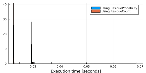
432         │       0.0    2.25097  …    2.40596        0.0

In the above examples, we indicate the type of each occurrence in the counting and the probability table to use. Also, it's possible for some measures as entropy and mutual information, to estimate the values only with the count table (without calculate the probability table). Estimating measures only with a ResidueCount table, when this is possible, should be faster than using a probability table.

Time_Pab = map(1:100) do x
    time = @elapsed mapcolpairfreq!(
        shannon_entropy,
        msa,
        Probabilities(ContingencyTable(Float64, Val{2}, UngappedAlphabet())),
    )
end

Time_Nab = map(1:100) do x
    time = @elapsed mapcolpairfreq!(
        shannon_entropy,
        msa,
        Frequencies(ContingencyTable(Float64, Val{2}, UngappedAlphabet())),
    )
end

using Plots
gr()

histogram(
    [Time_Pab Time_Nab],
    labels = ["Using ResidueProbability" "Using ResidueCount"],
    xlabel = "Execution time [seconds]",
)

Corrected Mutual Information

MIToS ships with two methods to easily calculate corrected mutual information. The first is the algorithm described in Buslje et al. [3]. This algorithm can be accessed through the buslje09 function and includes:

Low count correction using AdditiveSmoothing
Sequence weighting after a hobohmI clustering [2]
Average Product Correction (APC) proposed by Dunn et al. [5], through the APC! function that takes a MI matrix.
Z score correction using the functions shuffle_msa! from the MSA module and zscore from the PairwiseListMatrices package.

MIToS.Information.buslje09 — Function

buslje09 takes a MSA and calculates a Z score and a corrected MI/MIp as described on Busjle et al. 2009.

keyword argument, type, default value and descriptions:

  - lambda      Float64   0.05    Low count value
  - clustering  Bool      true    Sequence clustering (Hobohm I)
  - threshold             62      Percent identity threshold for clustering
  - maxgap      Float64   0.5     Maximum fraction of gaps in positions included in calculation
  - apc         Bool      true    Use APC correction (MIp)
  - samples     Int       100     Number of samples for Z-score
  - fixedgaps   Bool      true    Fix gaps positions for the random samples
  - alphabet    ResidueAlphabet UngappedAlphabet()  Residue alphabet to be used

This function returns:

  - Z score
  - MI or MIp

source

The second, implemented in the BLMI function, has the same corrections that the above algorithm, but use BLOSUM62 pseudo frequencies. This function is slower than buslje09 (at the same number of samples), but gives better performance (for structural contact prediction) when the MSA has less than 400 clusters after a Hobohm I at 62% identity.

MIToS.Information.BLMI — Function

BLMI takes an MSA and calculates a Z score (ZBLMI) and a corrected MI/MIp as described on Busjle et al. 2009 but using using BLOSUM62 pseudo frequencies instead of a fixed pseudocount.

Keyword argument, type, default value and descriptions:

  - beta        Float64   8.512   β for BLOSUM62 pseudo frequencies
  - lambda      Float64   0.0     Low count value
  - threshold             62      Percent identity threshold for sequence clustering (Hobohm I)
  - maxgap      Float64   0.5     Maximum fraction of gaps in positions included in calculation
  - apc         Bool      true    Use APC correction (MIp)
  - samples     Int       50      Number of samples for Z-score
  - fixedgaps   Bool      true    Fix gaps positions for the random samples

This function returns:

  - Z score (ZBLMI)
  - MI or MIp using BLOSUM62 pseudo frequencies (BLMI/BLMIp)

References

Buslje, Cristina Marino, et al. "Correction for phylogeny, small number of observations and data redundancy improves the identification of coevolving amino acid pairs using mutual information." Bioinformatics 25.9 (2009): 1125-1131.

source

Example: Estimating corrected MI from an MSA

using MIToS.MSA
using MIToS.Information

msa = read_file(
    "https://raw.githubusercontent.com/diegozea/MIToS.jl/master/docs/data/PF18883.stockholm.gz",
    Stockholm,
)
ZMIp, MIp = buslje09(msa)
ZMIp

107×107 Named PairwiseListMatrices.PairwiseListMatrix{Float64, false, Vector{Float64}}
Col1 ╲ Col2 │         57          58  …         431         432
────────────┼──────────────────────────────────────────────────
57          │        NaN     3.25274  …     1.38945    -1.38567
58          │    3.25274         NaN       -2.08538     4.56056
59          │    5.04975     3.23443        2.97155     -2.7079
60          │    1.38393     3.33905        -3.2956     1.39512
61          │    3.51849     1.02903       0.505697    -1.69826
64          │    1.17778     4.11793       -2.63834     5.06113
65          │   0.101109    -1.15235       0.836405     -2.6048
66          │   0.264063     4.73749       -3.05505      2.7723
⋮                      ⋮           ⋮  ⋱           ⋮           ⋮
423         │   0.367235    -1.75688      -0.223408   -0.700785
424         │    1.49777     1.40958       -2.50772     4.30845
427         │    1.14857   -0.376888         2.0029    0.170692
428         │   -2.05199     2.28319       -1.30895     3.03717
429         │   0.231057    -1.23643        6.09982    -0.72507
430         │   -1.40566     2.68801       -2.55912     5.80094
431         │    1.38945    -2.08538            NaN    -3.08604
432         │   -1.38567     4.56056  …    -3.08604         NaN

ZBLMIp, BLMIp = BLMI(msa)
ZBLMIp

107×107 Named PairwiseListMatrices.PairwiseListMatrix{Float64, false, Vector{Float64}}
Col1 ╲ Col2 │           57            58  …           431           432
────────────┼──────────────────────────────────────────────────────────
57          │          NaN    -0.0058753  …      0.054706   -0.00724753
58          │   -0.0058753           NaN      -0.00230327     0.0093646
59          │  -0.00462501     0.0177384        0.0716935   -0.00916293
60          │   -0.0385254     0.0114635       -0.0411778    0.00585093
61          │    0.0076633   -0.00767814        0.0146958   -0.00519354
64          │    0.0070737    0.00620751        -0.005128     0.0122708
65          │    -0.046307    -0.0287545       0.00846159    -0.0071145
66          │    -0.018272     0.0306033       -0.0277811    0.00521656
⋮                        ⋮             ⋮  ⋱             ⋮             ⋮
423         │     0.030699    -0.0166871       -0.0186436   -0.00203097
424         │    0.0653332    -0.0104712       -0.0142883    0.00839156
427         │    0.0409193    -0.0109902        0.0254383  -0.000165967
428         │   -0.0293523     0.0176844      -0.00865934     0.0105738
429         │    0.0123588    -0.0182636        0.0861102   -0.00345761
430         │   -0.0202489   -0.00581871       -0.0176394     0.0242715
431         │     0.054706   -0.00230327              NaN   -0.00883419
432         │  -0.00724753     0.0093646  …   -0.00883419           NaN

Visualize Mutual Information

You can use the function of the Plots package to visualize the Mutual Information (MI) network between residues. As an example, we are going to visualize the MI between residues of the Pfam domain PF18883. The heatmap is the simplest way to visualize the values of the Mutual Information matrix.

using Plots
gr()

heatmap(ZMIp, yflip = true)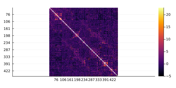

ZMIp is a Z score of the corrected MIp against its distribution on a random MSA (shuffling the residues in each sequence), so pairs with highest values are more likely to coevolve. Here, we are going to use the top 1% pairs of MSA columns.

using PairwiseListMatrices # to use getlist
using Statistics # to use quantile

threshold = quantile(getlist(ZMIp), 0.99)

6.967400960553533

ZMIp[ZMIp.<threshold] .= NaN
heatmap(ZMIp, yflip = true)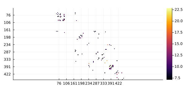

We are going to calculate the cMI (cumulative mutual information) value of each node. Where cMI is a mutual information score per position that characterizes the extent of mutual information "interactions" in its neighbourhood. This score is calculated as the sum of MI values above a certain threshold for every amino acid pair where the particular residue appears. This value defines to what degree a given amino acid takes part in a mutual information network and we are going to indicate it using the node color. To calculate cMI we are going to use the cumulative function:

cMI = cumulative(ZMIp, threshold)

1×107 Named Matrix{Float64}
Function ╲ Col2 │      57       58       59  …      430      431      432
────────────────┼────────────────────────────────────────────────────────
cumulative      │     0.0      0.0      0.0  …      0.0      0.0      0.0